Check overdispersion

code

Stats

binomial and poisson overdispersion checks

Author

Zhenglei Gao

Published

November 11, 2024

https://cran.r-project.org/web/packages/aods3/
https://cran.r-project.org/web/packages/dispmod/dispmod.pdf
https://cran.r-project.org/web/packages/DHARMa/vignettes/DHARMa.html
performance::check_overdispersion
https://stats.stackexchange.com/questions/409490/how-do-i-carry-out-a-significance-test-with-tarones-z-statistic
https://rpubs.com/cakapourani/beta-binomial

Overdipersion from package performance

library(glmmTMB)
data(Salamanders)
m <- glm(count ~ spp + mined, family = poisson, data = Salamanders)
check_overdispersion(m)

m <- glmmTMB(
  count ~ mined + spp + (1 | site),
  family = poisson,
  data = Salamanders
)
check_overdispersion(m)

library(dispmod)

Warning: package 'dispmod' was built under R version 4.4.2

help(glm.binomial.disp)

starting httpd help server ... done

data(orobanche)
mod <- glm(cbind(germinated, seeds-germinated) ~ host*variety, data = orobanche,
           family = binomial(logit))
summary(mod)


Call:
glm(formula = cbind(germinated, seeds - germinated) ~ host * 
    variety, family = binomial(logit), data = orobanche)

Coefficients:
                      Estimate Std. Error z value Pr(>|z|)  
(Intercept)            -0.4122     0.1842  -2.238   0.0252 *
hostCuke                0.5401     0.2498   2.162   0.0306 *
varietyO.a75           -0.1459     0.2232  -0.654   0.5132  
hostCuke:varietyO.a75   0.7781     0.3064   2.539   0.0111 *
---
Signif. codes:  0 '***' 0.001 '**' 0.01 '*' 0.05 '.' 0.1 ' ' 1

(Dispersion parameter for binomial family taken to be 1)

    Null deviance: 98.719  on 20  degrees of freedom
Residual deviance: 33.278  on 17  degrees of freedom
AIC: 117.87

Number of Fisher Scoring iterations: 4

mod.disp <- glm.binomial.disp(mod)


Binomial overdispersed logit model fitting...
Iter.  1  phi: 0.02371848 
Iter.  2  phi: 0.0248754 
Iter.  3  phi: 0.02493477 
Iter.  4  phi: 0.02493781 
Iter.  5  phi: 0.02493797 
Iter.  6  phi: 0.02493797 
Converged after 6 iterations. 
Estimated dispersion parameter: 0.02493797 

Call:
glm(formula = cbind(germinated, seeds - germinated) ~ host * 
    variety, family = binomial(logit), data = orobanche, weights = disp.weights)

Coefficients:
                      Estimate Std. Error z value Pr(>|z|)  
(Intercept)           -0.46533    0.24387  -1.908   0.0564 .
hostCuke               0.51023    0.33472   1.524   0.1274  
varietyO.a75          -0.07009    0.31146  -0.225   0.8220  
hostCuke:varietyO.a75  0.81956    0.43522   1.883   0.0597 .
---
Signif. codes:  0 '***' 0.001 '**' 0.01 '*' 0.05 '.' 0.1 ' ' 1

(Dispersion parameter for binomial family taken to be 1)

    Null deviance: 47.243  on 20  degrees of freedom
Residual deviance: 18.442  on 17  degrees of freedom
AIC: 65.578

Number of Fisher Scoring iterations: 4

summary(mod.disp)


Call:
glm(formula = cbind(germinated, seeds - germinated) ~ host * 
    variety, family = binomial(logit), data = orobanche, weights = disp.weights)

Coefficients:
                      Estimate Std. Error z value Pr(>|z|)  
(Intercept)           -0.46533    0.24387  -1.908   0.0564 .
hostCuke               0.51023    0.33472   1.524   0.1274  
varietyO.a75          -0.07009    0.31146  -0.225   0.8220  
hostCuke:varietyO.a75  0.81956    0.43522   1.883   0.0597 .
---
Signif. codes:  0 '***' 0.001 '**' 0.01 '*' 0.05 '.' 0.1 ' ' 1

(Dispersion parameter for binomial family taken to be 1)

    Null deviance: 47.243  on 20  degrees of freedom
Residual deviance: 18.442  on 17  degrees of freedom
AIC: 65.578

Number of Fisher Scoring iterations: 4

mod.disp$dispersion

[1] 0.02493797

library(DHARMa)

Warning: package 'DHARMa' was built under R version 4.4.2

This is DHARMa 0.4.7. For overview type '?DHARMa'. For recent changes, type news(package = 'DHARMa')

citation("DHARMa")

To cite package 'DHARMa' in publications use:

  Hartig F (2024). _DHARMa: Residual Diagnostics for Hierarchical
  (Multi-Level / Mixed) Regression Models_. R package version 0.4.7,
  <https://CRAN.R-project.org/package=DHARMa>.

A BibTeX entry for LaTeX users is

  @Manual{,
    title = {DHARMa: Residual Diagnostics for Hierarchical (Multi-Level / Mixed)
Regression Models},
    author = {Florian Hartig},
    year = {2024},
    note = {R package version 0.4.7},
    url = {https://CRAN.R-project.org/package=DHARMa},
  }

Tarone’s test

#' Tarone's Z Test
#' 
#' Tests the goodness of fit of the binomial distribution.
#' 
#' @param M Counts
#' @param N Trials
#' 
#' @return a \code{htest} object
#' 
#' @author \href{https://stats.stackexchange.com/users/173082/reinstate-monica}{Ben O'Neill}
#' @references \url{https://stats.stackexchange.com/a/410376/6378} and
#' R. E. TARONE, Testing the goodness of fit of the binomial distribution, Biometrika, Volume 66, Issue 3, December 1979, Pages 585–590, \url{https://doi.org/10.1093/biomet/66.3.585}
#' @importFrom stats pnorm
#' @export
#' @examples 
#'  #Generate example data
#' N <- c(30, 32, 40, 28, 29, 35, 30, 34, 31, 39)
#' M <- c( 9, 10, 22, 15,  8, 19, 16, 19, 15, 10)
#' Tarone.test(N, M)
Tarone.test <- function(N, M) {
  
  #Check validity of inputs
  if(!(all(N == as.integer(N)))) { stop("Error: Number of trials should be integers"); }
  if(min(N) < 1) { stop("Error: Number of trials should be positive"); }
  if(!(all(M == as.integer(M)))) { stop("Error: Count values should be integers"); }
  if(min(M) < 0) { stop("Error: Count values cannot be negative"); }
  if(any(M > N)) { stop("Error: Observed count value exceeds number of trials"); }
  
  #Set description of test and data
  method      <- "Tarone's Z test";
  data.name   <- paste0(deparse(substitute(M)), " successes from ", 
                        deparse(substitute(N)), " trials");
  
  #Set null and alternative hypotheses
  null.value  <- 0;
  attr(null.value, "names") <- "dispersion parameter";
  alternative <- "greater";
  
  #Calculate test statistics
  estimate    <- sum(M)/sum(N);
  attr(estimate, "names") <- "proportion parameter";
  S           <- ifelse(estimate == 1, sum(N),
                        sum((M - N*estimate)^2/(estimate*(1 - estimate))));
  statistic   <- (S - sum(N))/sqrt(2*sum(N*(N-1))); 
  attr(statistic, "names") <- "z";
  
  #Calculate p-value
  p.value     <- 2*pnorm(-abs(statistic), 0, 1);
  attr(p.value, "names") <- NULL;
  
  #Create htest object
  TEST        <- list(method = method, data.name = data.name,
                      null.value = null.value, alternative = alternative,
                      estimate = estimate, statistic = statistic, p.value = p.value);
  class(TEST) <- "htest";
  TEST; 
}

#Generate example data
N <- c(30, 32, 40, 28, 29, 35, 30, 34, 31, 39);
M <- c( 9, 10, 22, 15,  8, 19, 16, 19, 15, 10);
#Apply Tarone's test to the example data
TEST <- Tarone.test(N, M);
TEST;


    Tarone's Z test

data:  M successes from N trials
z = 2.5988, p-value = 0.009355
alternative hypothesis: true dispersion parameter is greater than 0
sample estimates:
proportion parameter 
           0.4359756

In this case we have a low p-value, so we find strong evidence to reject the null hypothesis of a binomial distribution in favour of the alternative of over-dispersion. We can fit the data to the beta-binomial model to estimate the dispersion parameter:

#Fit the example data to a beta-binomial distribution
DATA <- data.frame(m=M,n=N)
library(VGAM)

Warning: package 'VGAM' was built under R version 4.4.2

Loading required package: stats4

Loading required package: splines

MODEL <- VGAM::vglm(cbind(DATA$m, DATA$n-DATA$m) ~ 1, betabinomial, trace = FALSE);
Coef(MODEL);

        mu        rho 
0.43507150 0.03355549

library(lme4)

Loading required package: Matrix

set.seed(101)

# "actual" data
intercept <- 0.1; slope <- 0.8
covariate <- runif(1000)
latent_response <- intercept + covariate*slope
observed_response <- rbinom(1000, prob=plogis(latent_response), size=10)
realdat <- data.frame(m = observed_response, n=rep(10,1000), x = covariate, grp = rep(1:100, each = 10))
null <- glmer(cbind(m, n-m) ~ x + (1|grp), data=realdat, family="binomial")

# parametric bootstrap with function from Ben's answer
sims <- replicate(1000,{ fakedat <- simulate(null)[[1]]; Tarone.test(rowSums(fakedat), fakedat[,1])$statistic })
obs <- Tarone.test(realdat$n, realdat$m)$statistic
# approximate one-tailed pval
sum(sims > obs)/length(sims)

[1] 0.52

hist(sims);abline(v=obs,col="red") #no evidence for overdispersion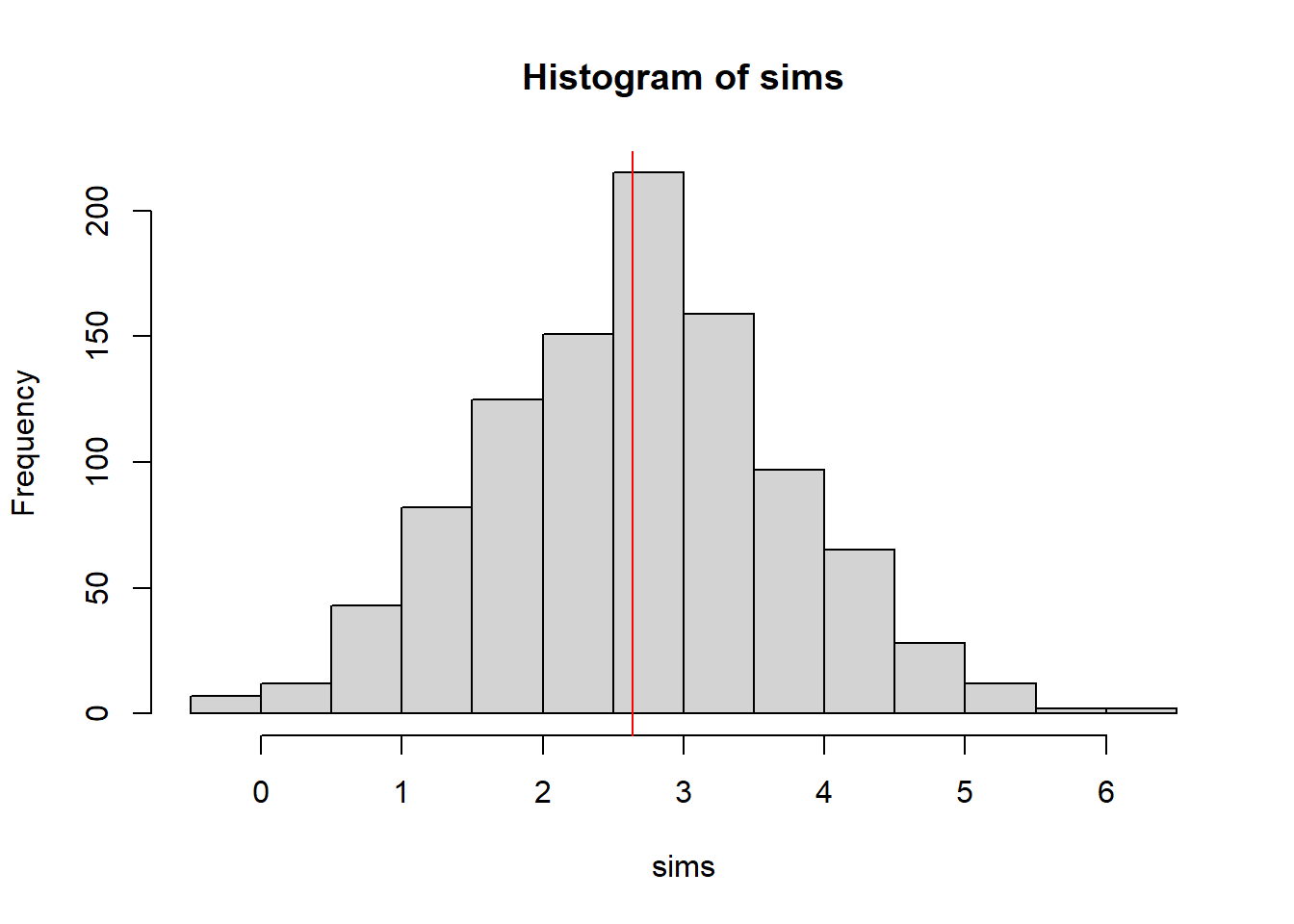

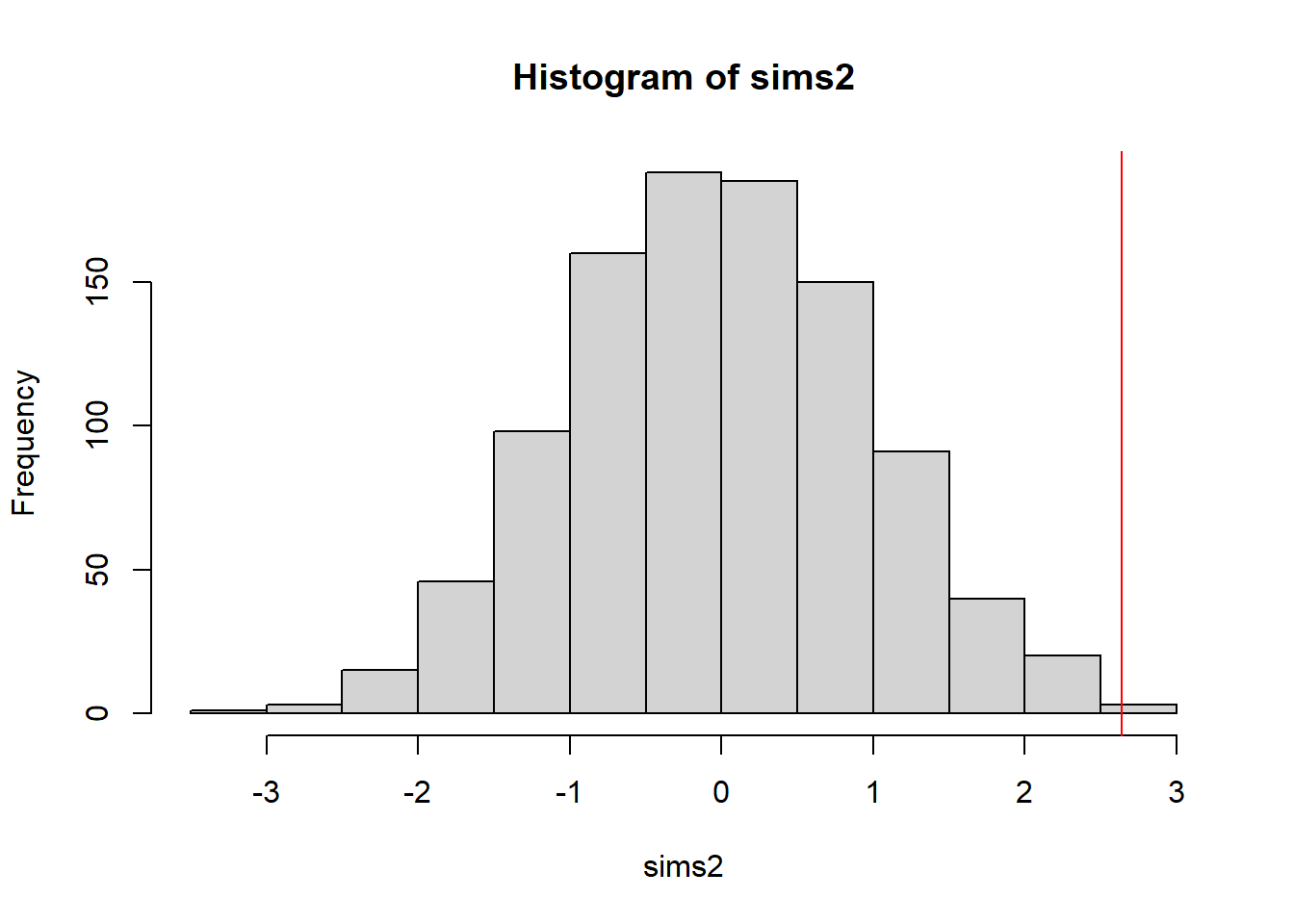
# what if covariate was not measured?
null2 <- glmer(cbind(n, n-m) ~ (1|grp), data=realdat, family="binomial")

boundary (singular) fit: see help('isSingular')

sims2 <- replicate(1000,{ fakedat <- simulate(null2)[[1]]; Tarone.test(rowSums(fakedat), fakedat[,1])$statistic })
sum(sims2 > obs)/length(sims2)

[1] 0.002

hist(sims2);abline(v=obs,col="red") #now appears to be evidence for overdispersion