Variance Component Analysis

VCA for fixed and mixed models

Author

Zhenglei Gao

Published

May 24, 2025

I realized during the analysis that variance components of mixed models can sum to more than 1. The issue is that in mixed models, fixed effects and random effects can be correlated, which creates non-additivity in variance decomposition. So I turned to MGA and try to understand.

Why Variance Components Can Sum to More Than 1

The non-additivity of variance components (why they can sum to more than 1) occurs due to several important statistical reasons:

1. Mathematical Explanation

When we decompose the total variance into components, we’re essentially trying to partition:

Var(Y) = Var(Xβ + Zu + ε)

Where: - Xβ represents fixed effects - Zu represents random effects - ε represents residuals

If the components were independent, we would have:

Var(Y) = Var(Xβ) + Var(Zu) + Var(ε)

However, in most real-world scenarios, fixed effects (Xβ) and random effects (Zu) are not independent. This leads to:

Var(Y) = Var(Xβ) + Var(Zu) + Var(ε) + 2*Cov(Xβ, Zu)

The covariance term is what creates the non-additivity.

2. Code Example to Demonstrate

Let’s create a simple example to show this:

library(lme4)

Loading required package: Matrix

# Create a demonstration
set.seed(123)
n <- 200
groups <- 20
group_id <- rep(1:groups, each = n/groups)

# Create predictor with between-group differences
x <- rnorm(n) + rep(rnorm(groups), each = n/groups)  # Predictor correlated with group
random_effect <- rnorm(groups)[group_id]  # Random group effect
y <- 2 + 3*x + random_effect + rnorm(n)  # Response with fixed and random effects

demo_data <- data.frame(y = y, x = x, group = factor(group_id))

# Fit model
demo_model <- lmer(y ~ x + (1|group), data = demo_data)

My old wy of using VCA

library(VCA)


Attaching package: 'VCA'

The following objects are masked from 'package:lme4':

    fixef, getL, ranef

fit <- anovaMM(y ~ x *(group), demo_data)
inf <- VCAinference(fit, VarVC=TRUE)
print(inf, what="VCA")




Inference from Mixed Model Fit
------------------------------

> VCA Result:
-------------

    [Fixed Effects]

   int      x 
1.9932 2.9997 


    [Variance Components]

  Name    DF      SS       MS     VC     %Total  SD     CV[%]   Var(VC)
1 total   64.0299                 1.8489 100     1.3598 63.1311 0.1089 
2 group   19      175.1819 9.2201 0.7608 41.1452 0.8722 40.4952 0.1028 
3 x:group 19      30.1765  1.5882 0.0713 3.8566  0.267  12.3978 0.0044 
4 error   160     162.7022 1.0169 1.0169 54.9982 1.0084 46.8186 0.0129 

Mean: 2.1539 (N = 200) 

Experimental Design: unbalanced  |  Method: ANOVA

# Calculate variance components
# 1. Total variance
total_var <- var(demo_data$y)

# 2. Fixed effects variance
fixed_pred <- predict(demo_model, re.form = NA)
fixed_var <- var(fixed_pred)

# 3. Random effects variance
vc <- VarCorr(demo_model)
random_var <- attr(vc$group, "stddev")^2

# 4. Residual variance
residual_var <- attr(vc, "sc")^2

# 5. Calculate correlation between fixed and random effects
random_effects <- lme4::ranef(demo_model)$group[,1][demo_data$group]
correlation <- cor(fixed_pred, random_effects)

# Results
components <- c(
  fixed = fixed_var / total_var,
  random = random_var / total_var,
  residual = residual_var / total_var,
  sum = (fixed_var + random_var + residual_var) / total_var
)

print("Variance components as proportion of total variance:")

[1] "Variance components as proportion of total variance:"

print(components)

             fixed random.(Intercept)           residual    sum.(Intercept) 
        0.90729780         0.03903374         0.05112009         0.99745163

print(paste("Correlation between fixed and random effects:", round(correlation, 3)))

[1] "Correlation between fixed and random effects: 0.014"

3. Why This Happens in Practice

Several practical reasons contribute to this phenomenon:

Confounding between predictors and groups:
- When predictors (fixed effects) are correlated with grouping variables
- Example: If certain active substances are used more in certain crops
Shared information:
- Fixed and random effects can explain some of the same variation
- This creates “double-counting” in variance decomposition
Model specification:
- The way we specify fixed vs. random effects affects their correlation
- Including group-level predictors can reduce this correlation
Estimation method:
- REML vs ML estimation can affect variance partitioning
- Shrinkage in random effects estimation

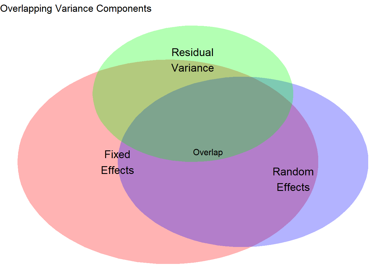
4. Visualization of Overlapping Variance

Here’s a visual representation:

# Create a visual representation of overlapping variance
library(ggplot2)
library(gridExtra)

# Create data for Venn diagram-like visualization
circle_data <- function(x0, y0, r, n = 100) {
  theta <- seq(0, 2*pi, length.out = n)
  data.frame(x = x0 + r*cos(theta), y = y0 + r*sin(theta))
}

# Create circles
fixed_circle <- circle_data(0, 0, 3)
random_circle <- circle_data(1.5, 0, 2.5)
residual_circle <- circle_data(0.5, 2, 2)

# Plot
p <- ggplot() +
  geom_polygon(data = fixed_circle, aes(x, y), fill = "red", alpha = 0.3) +
  geom_polygon(data = random_circle, aes(x, y), fill = "blue", alpha = 0.3) +
  geom_polygon(data = residual_circle, aes(x, y), fill = "green", alpha = 0.3) +
  annotate("text", x = -1, y = 0, label = "Fixed\nEffects", size = 5) +
  annotate("text", x = 2.5, y = -0.5, label = "Random\nEffects", size = 5) +
  annotate("text", x = 0.5, y = 3, label = "Residual\nVariance", size = 5) +
  annotate("text", x = 0.8, y = 0.3, label = "Overlap", size = 4) +
  theme_void() +
  labs(title = "Overlapping Variance Components")

print(p)

5. Handling Non-Additivity

To handle this non-additivity, you can:

Report unadjusted components with acknowledgment of overlap
Adjust components to sum to 100% (as in the previous code)
Use alternative metrics like R² marginal and conditional
Orthogonalize predictors to reduce correlation with grouping variables

Would you like me to: 1. Add more detailed mathematical explanations? 2. Create a more specific example with your data? 3. Show alternative variance decomposition approaches? 4. Add code for reducing the correlation between fixed and random effects? 5. Provide guidance on interpreting overlapping variance components?