Cluster Analysis Refresher

Simple cluster analysis

Warning

To be written.

I started working on a project clustering a trait database so that I can get up to 15 clusters of species groups. Hence I am refreshing on the potential algorithms I could use.

Algorithms

There are different types of clustering alogrithm with different distance measures, including density-based, distribution-based, centroid-based, hierarchical-based, model-based.

• The common 4 distances measures are Enclidaen, Manhattan, Correlation and Eisen.

We focus on a few for the moment.

• Partitioning Clustering
  • K-means clustering (centroid-based)
  • K-Medoids (PAM)
  • CLARA
• DBSCAN (density-based spatial clustering of applications with noise)
• Hierarchical Clustering
  • • Agglomerative Hierarchy clustering algorithm
      
• Spectral Clustering

Cluster GoF (clValid)

• Internal: the connectivity, the silhouette coefficient and the Dunn index
• Stability: average proportion of non-overlap, average distance, average distance between means, figure of metrit.

CLARA

CLARA is used in another python ML project. Compared to k-means clustering, CLARA is an extention of k-medoids methods to deal with large data. It is achieved by iterative sampling and then clusterting.

Using tidymodels or tidy pipeline

DBSCAN

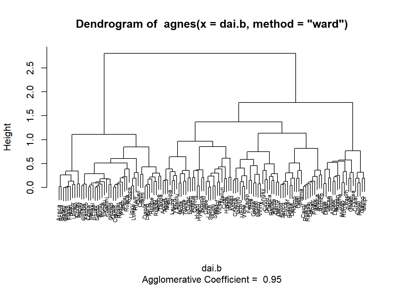
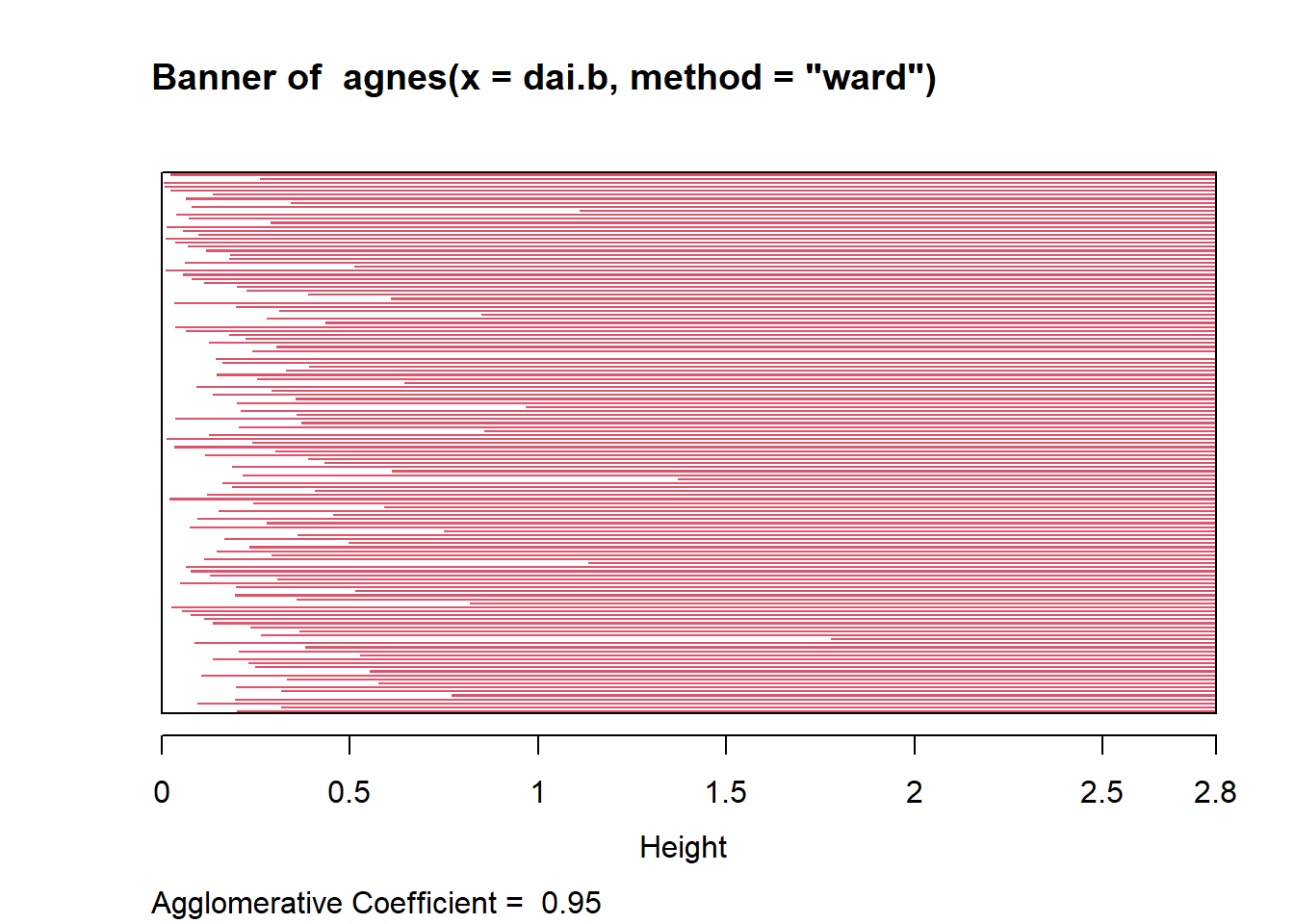
Agglomerative hierarchy clustering

library(cluster)
data(plantTraits)

## Calculation of a dissimilarity matrix

dai.b <- daisy(plantTraits,
               type = list(ordratio = 4:11, symm = 12:13, asymm = 14:31))

## Hierarchical classification
agn.trts <- agnes(dai.b, method="ward")
plot(agn.trts, which.plots = 2, cex= 0.6)

plot(agn.trts, which.plots = 1)

cutree6 <- cutree(agn.trts, k=6)
cutree6
#>   [1] 1 1 2 2 3 4 4 2 3 5 5 2 2 1 5 4 6 2 6 1 5 4 3 2 2 3 2 1 4 6 6 6 6 2 5 6 3
#>  [38] 5 4 3 5 2 2 6 1 6 1 1 3 4 4 3 3 3 6 2 5 2 2 2 6 5 5 4 4 6 2 6 2 6 3 6 2 2
#>  [75] 4 2 4 2 5 4 5 4 5 5 5 4 2 2 1 2 3 3 6 6 6 6 2 6 6 3 3 6 6 6 6 6 6 5 5 4 5
#> [112] 6 6 2 6 4 6 6 2 3 4 6 6 3 6 2 3 6 1 5 2 4 2 3 3 3

## Principal Coordinate Analysis
cmdsdai.b <- cmdscale(dai.b, k=6)
plot(cmdsdai.b[, 1:2], asp = 1, col = cutree6)