   (Intercept) diagnosesevere        drugnew           time   drugnew:time
   -0.02798843    -1.31391092    -0.05960381     0.48241209     1.01744498
summary(dep_gee)
 GEE:  GENERALIZED LINEAR MODELS FOR DEPENDENT DATA
 gee S-function, version 4.13 modified 98/01/27 (1998)

Model:
 Link:                      Logit
 Variance to Mean Relation: Binomial
 Correlation Structure:     Independent

Call:
gee(formula = depression ~ diagnose + drug * time, id = id, data = dat,
    family = binomial, corstr = "independence")

Summary of Residuals:
        Min          1Q      Median          3Q         Max
-0.94844242 -0.40683252  0.05155758  0.38830952  0.80242231


Coefficients:
                  Estimate Naive S.E.    Naive z Robust S.E.   Robust z
(Intercept)    -0.02798843  0.1627083 -0.1720160   0.1741865 -0.1606808
diagnosesevere -1.31391092  0.1453432 -9.0400569   0.1459845 -9.0003423
drugnew        -0.05960381  0.2205812 -0.2702126   0.2285385 -0.2608042
time            0.48241209  0.1139224  4.2345663   0.1199350  4.0222784
drugnew:time    1.01744498  0.1874132  5.4288855   0.1876938  5.4207709

Estimated Scale Parameter:  0.9854113
Number of Iterations:  1

Working Correlation
     [,1] [,2] [,3]
[1,]    1    0    0
[2,]    0    1    0
[3,]    0    0    1
res <-glm(depression ~ diagnose + drug*time,data = dat,family = quasibinomial)summary(res)
Call:
glm(formula = depression ~ diagnose + drug * time, family = quasibinomial,
    data = dat)

Coefficients:
               Estimate Std. Error t value Pr(>|t|)
(Intercept)    -0.02799    0.16271  -0.172    0.863
diagnosesevere -1.31391    0.14534  -9.040  < 2e-16 ***
drugnew        -0.05960    0.22058  -0.270    0.787
time            0.48241    0.11392   4.235 2.50e-05 ***
drugnew:time    1.01744    0.18741   5.429 7.09e-08 ***
---
Signif. codes:  0 '***' 0.001 '**' 0.01 '*' 0.05 '.' 0.1 ' ' 1

(Dispersion parameter for quasibinomial family taken to be 0.9854187)

    Null deviance: 1411.9  on 1019  degrees of freedom
Residual deviance: 1161.9  on 1015  degrees of freedom
AIC: NA

Number of Fisher Scoring iterations: 4
The “Estimated Scale Parameter” is reported as 0.9854113 = the dispersion parameter = similar to what is reported (Dispersion parameter for quasibinomial family taken to be 0.9854187) when running glm() with family = quasibinomial in order to model over-dispersion.
dep_gee2 <-gee(depression ~ diagnose + drug*time,data = dat, id = id, family = binomial,corstr ="exchangeable")
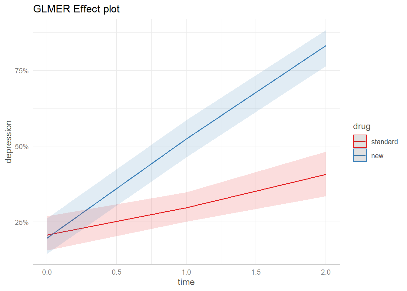
You are calculating adjusted predictions on the population-level (i.e.
  `type = "fixed"`) for a *generalized* linear mixed model.
  This may produce biased estimates due to Jensen's inequality. Consider
  setting `bias_correction = TRUE` to correct for this bias.
  See also the documentation of the `bias_correction` argument.
library(emmeans) # version 1.8.4-1
Warning: package 'emmeans' was built under R version 4.4.2
Welcome to emmeans.
Caution: You lose important information if you filter this package's results.
See '? untidy'
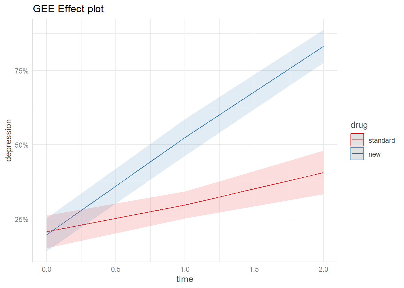
emm_out <-emmeans(dep_gee2, specs =c("time", "drug"), at =list(diagnose ="severe"), cov.keep ="time", regrid ="response") %>%as.data.frame()library(ggplot2) # version 3.4.1ggplot(emm_out) +aes(x = time, y = prob, color = drug, fill = drug) +geom_line() +geom_ribbon(aes(ymin = asymp.LCL, ymax = asymp.UCL, color =NULL), alpha =0.15) +scale_color_brewer(palette ="Set1") +scale_fill_brewer(palette ="Set1", guide =NULL) +scale_y_continuous(labels = scales::percent) +theme_ggeffects() +labs(title ="GEE Effect plot", y ="depression")
library(geepack) # version 1.3.9
Warning: package 'geepack' was built under R version 4.4.2