In this article, I will try to analyze percentage data as proportions, using log-logistic model with quasibinomial and nonlinear fit to the log-logistic cumulative distribution function (CDF) curves.
Proportional data where the denominator (e.g. maximum possible number of presence for a given response type) is not known can be modeled using a Beta distribution. Binomial-logit-Normal model with observation-level random effects can also be applied to proportions to handle over-dispersion, similarly, quasibinomial models.
For quasibinomial, an additional method is to add subject or individual or treatment group level random effect, that way additional noise is added to the model and can count for the spread of the data in addition to the quasi-binomial variance. However, there is no direct R functions available to calculate all the associated uncertainties, post-processing must be implemented manually. Therefore, the chance of that becoming a standard approach is very low.
The data is generated in two ways, one is based on the logistic CDF with added noise, the other is just using binomial sampling. For the latter, the sample size information is excluded from the final dataset to mimic the percentage data characteristics. We can also generate over-dispersed binomial data following the steps described here or here
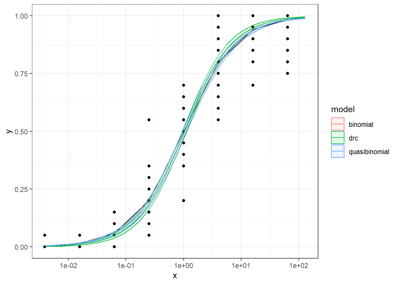
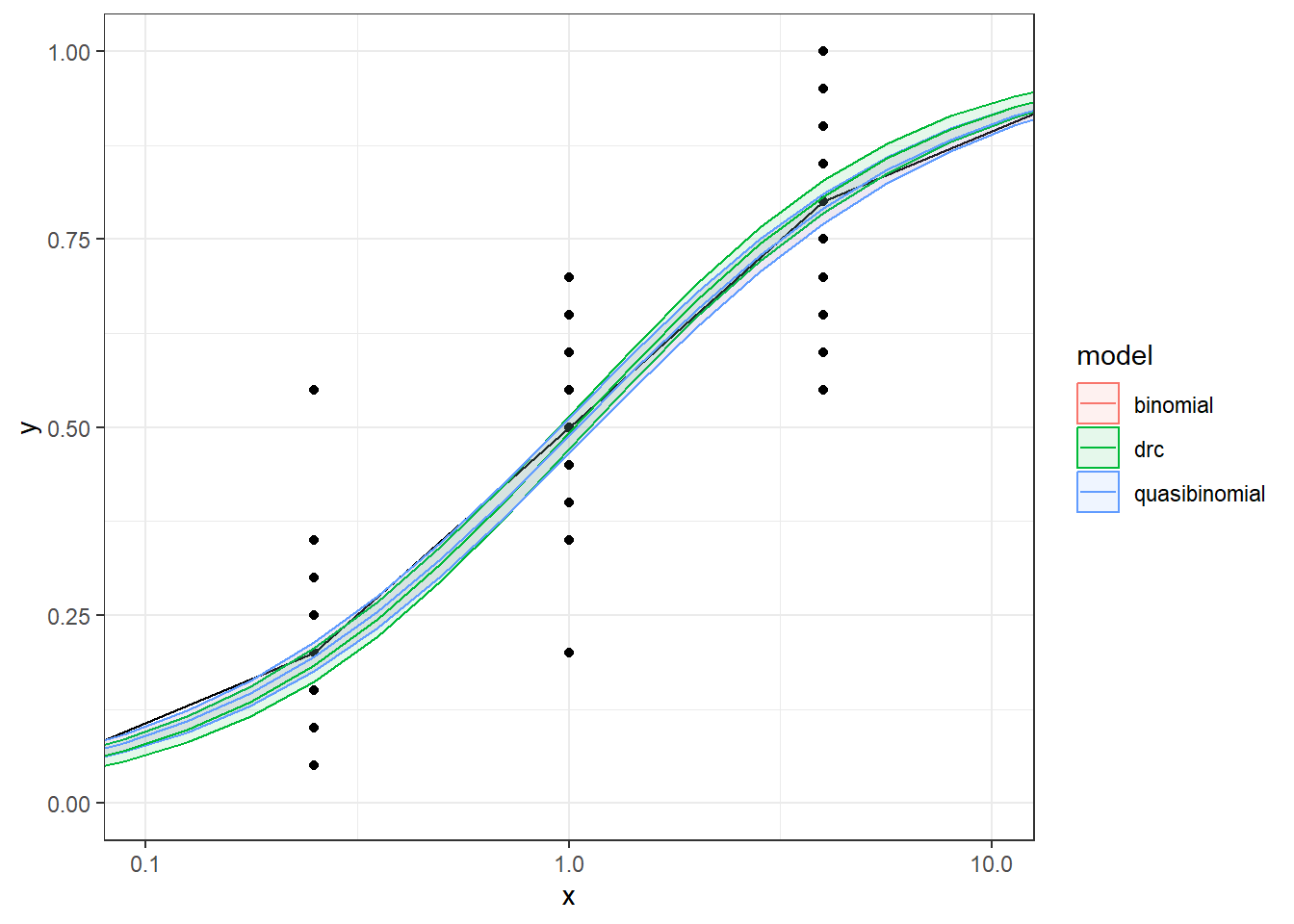
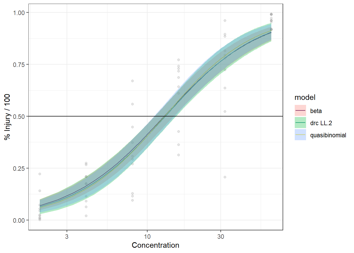
We are comparing the 3 methods with different data generation scheme.
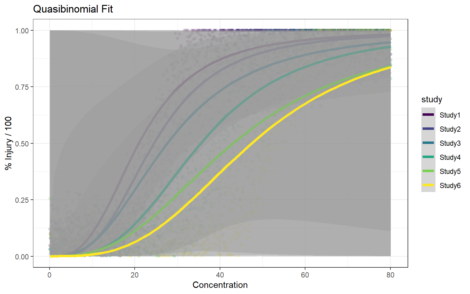
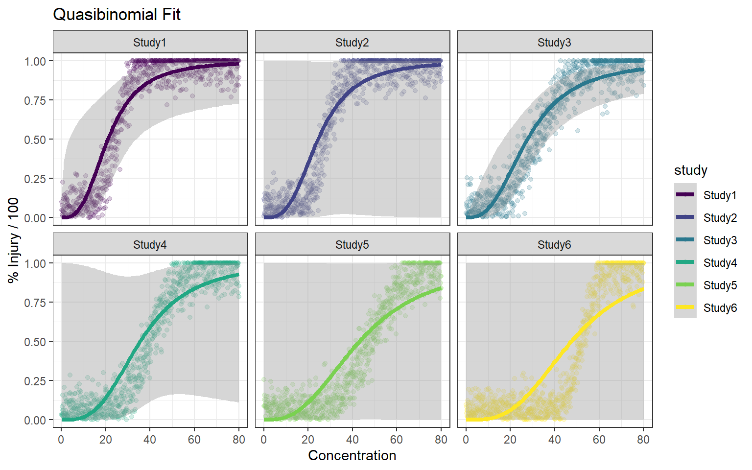
Method A: simple quasi binomial
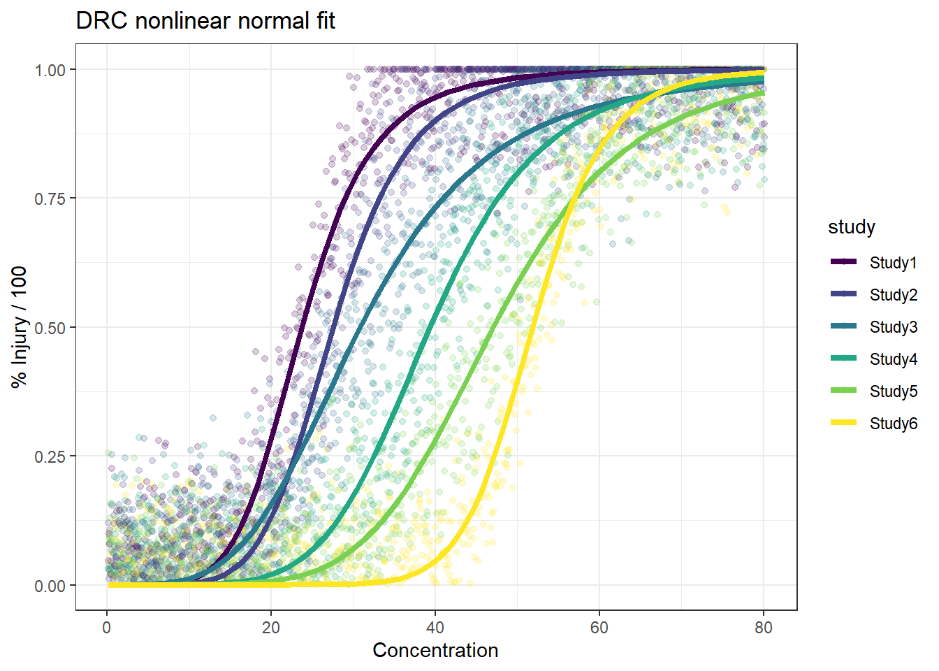
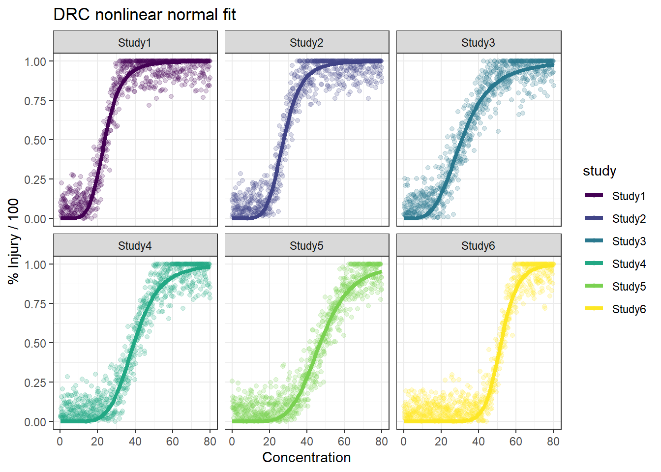
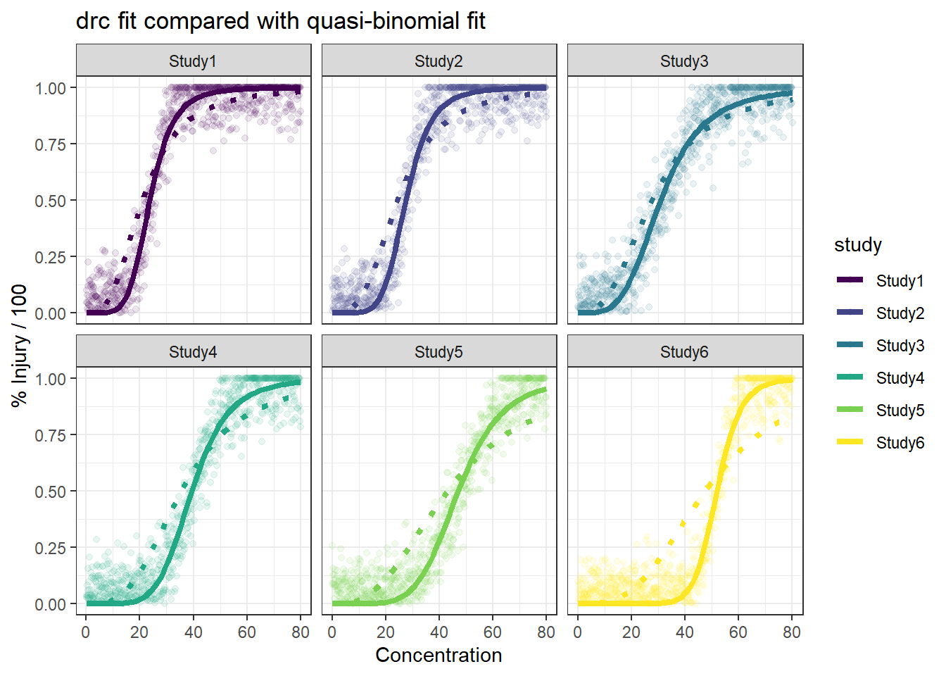
Method B: drc with normal spread around logistic CDF
Method B1: quasi-binomial with random effect (MASS::glmmPQL(percentages/100~ conc,random=~1|conc,family="quasibinomial",data=data))
Method C:
The conclusions are:
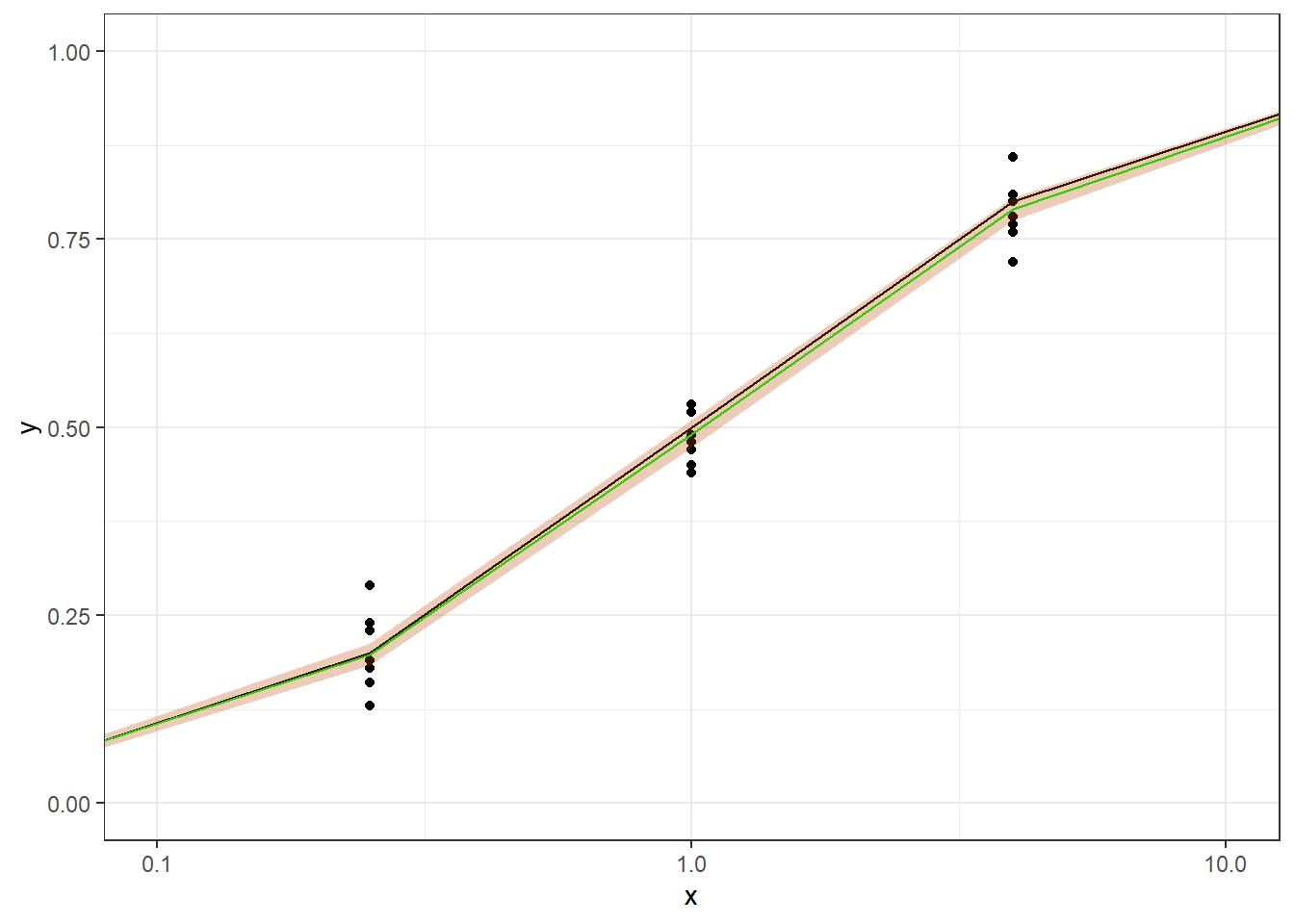
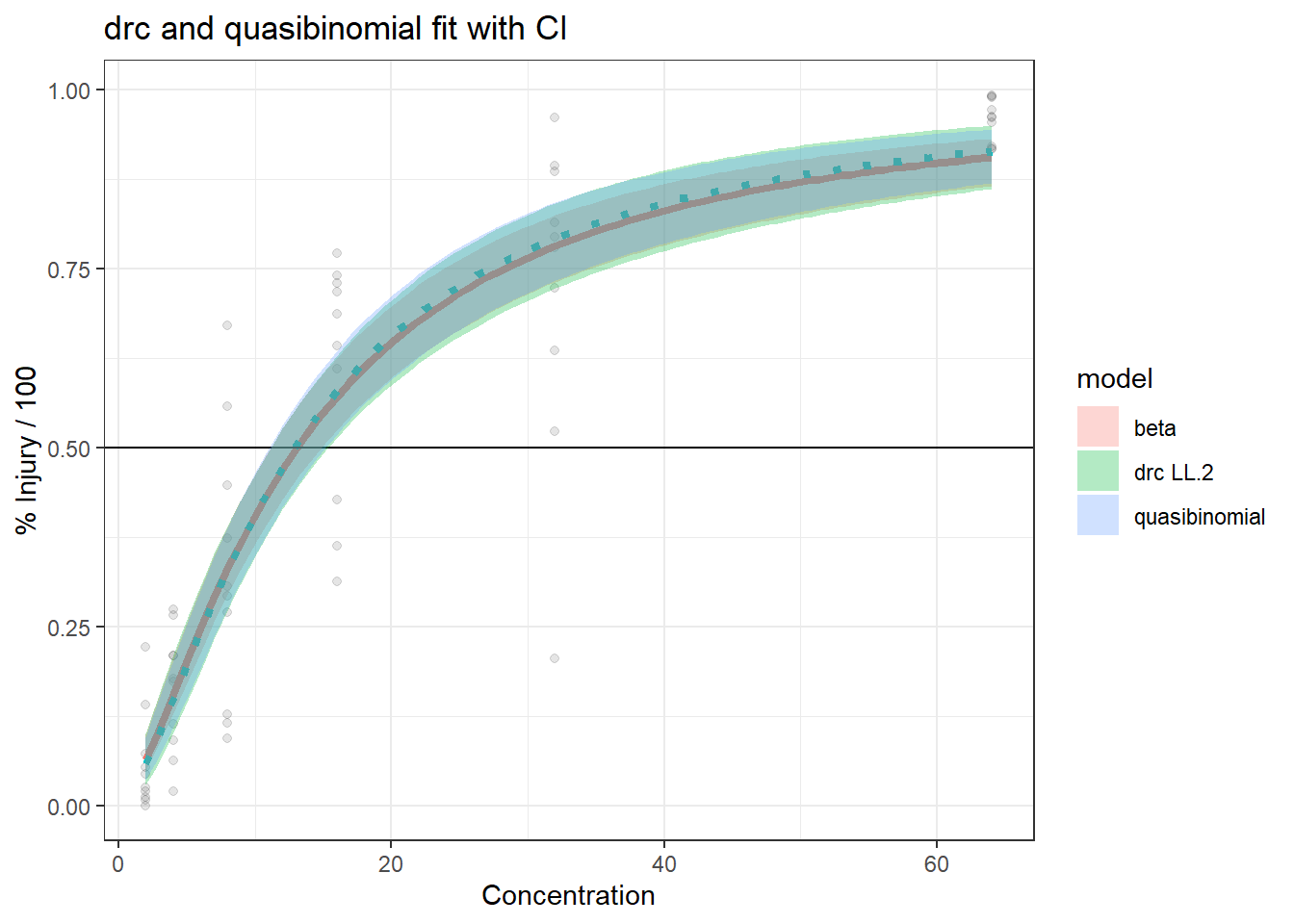
For the data generated based on logistic CDF, the standard DRC approach fit the data much better. In terms of EC50 estimation, and the fit of the curve.
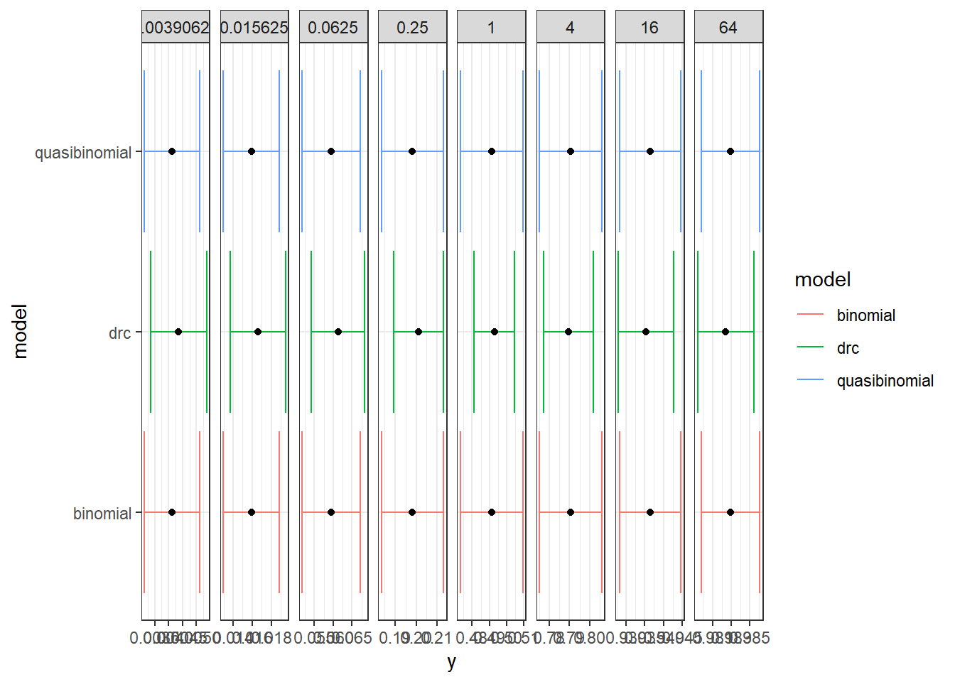
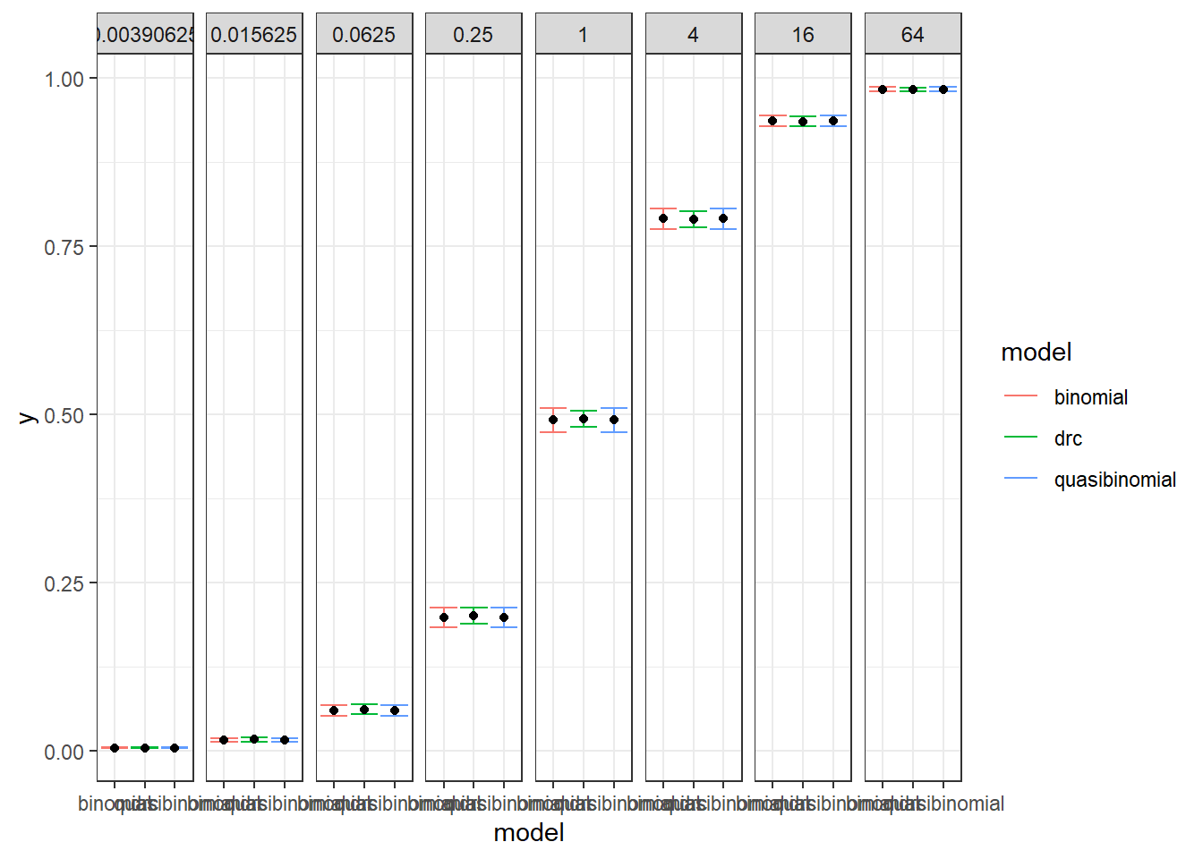
For the data generated using binomial sampling, the examined approaches are similar, in terms of both EC50 estimation and the curve estimation.
Data generated using the logistic CDF.
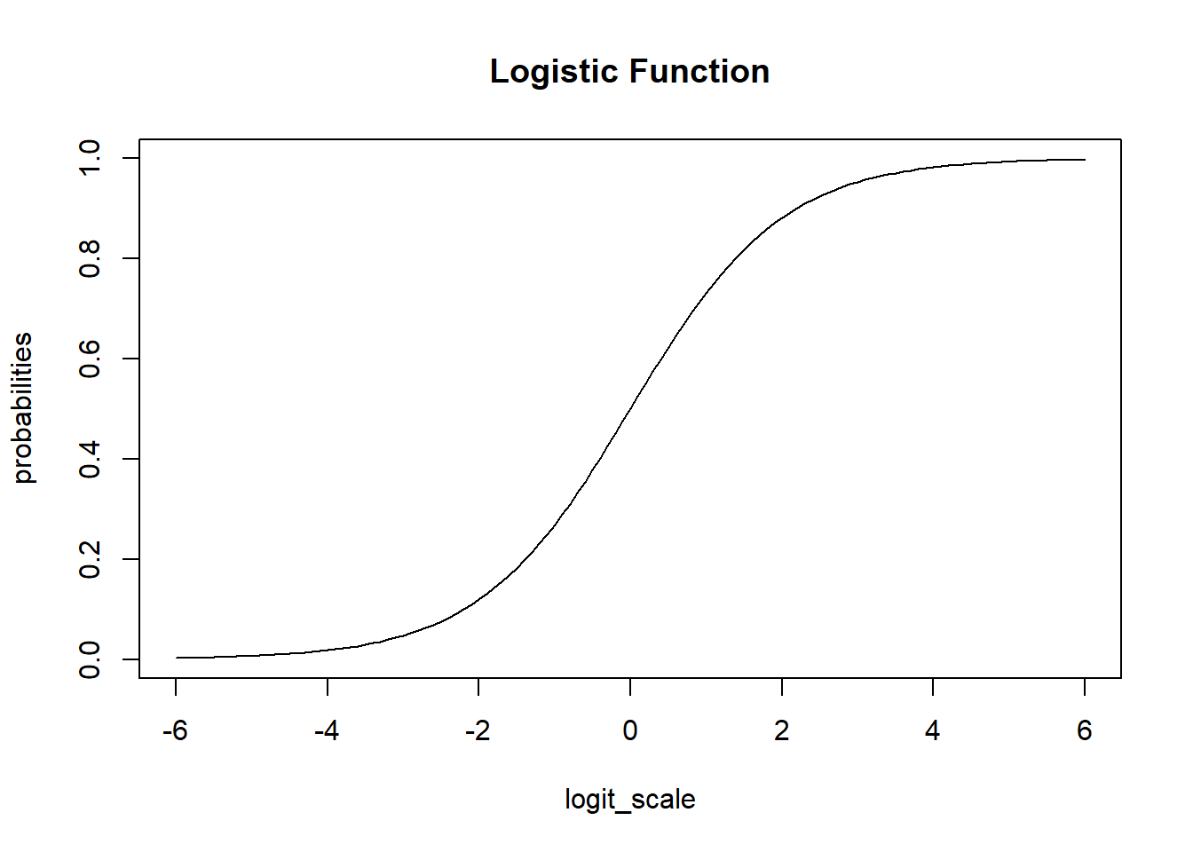
The data is generated using the cumulative function for logistic distribution. Note that the logistic function is just an inverse logit (\(\log(p/(1-p))\)) function in R. The code is modified based on this blog post. \[F(x;\mu,s) = \frac{1}{2} + \frac{1}{2} \tanh((x-\mu)/2s) = \frac{1}{1+e^{-(x-\mu)/s}}\]
where, \(\tanh(x) = \frac{\sinh(x)}{\cosh(x)} = \frac{e^x - e^{-x}}{e^x + e^{-x}}\), is the hyperbolic tangent function that maps real numbers to the range between -1 and 1.
Quantile of the CDF is then \(\mu+s\log(\frac{p}{1-p})\), therefore, the EC50 should be \(\mu\) or \(\exp(\mu)\).
Random noises are added afterwards to the logistic distribution CDF.
We simulate \(n\) studies over concentration \(x\), denoted, \(X_{1}, X_{2}, …, X_{n}\) for \(k\) study \(X=(x_{1}, x_{2}, …, x_{k})\), where \(k\) is the number of different studies with different \(\mu\) and \(\sigma\).
Let’s say there are \(k=6\) study groups with the following parameter sets, \(\mu = \{9,2,3,5,7,5\}\) and \(s=\{2,2,4,3,4,2\}\)
generate_logit_cdf <-function(mu, s, sigma_y=0.1, x=seq(-5,20,0.1)) { x_ms <- (x-mu)/s y <-0.5+0.5*tanh(x_ms) y <-abs(y +rnorm(length(x), 0, sigma_y)) ix <-which(y>=1.0)if(length(ix)>=1) { y[ix] <-1.0 }return(y)}tanh(0)
[1] 0
set.seed(424242)x <-seq(-5,15,0.025) mu_vec <-c(1,2,3,5,7,8) # 6 Studiesidx <-sapply(mu_vec,function(mu) which(x==mu))s_vec <-c(2,2,4,3,4,2)# Synthetic Study IDstudies_df<-mapply(generate_logit_cdf, mu_vec, s_vec, MoreArgs =list(x=x))# Give them namescolnames(studies_df) <-c("Study1", "Study2", "Study3", "Study4", "Study5", "Study6")dim(studies_df)
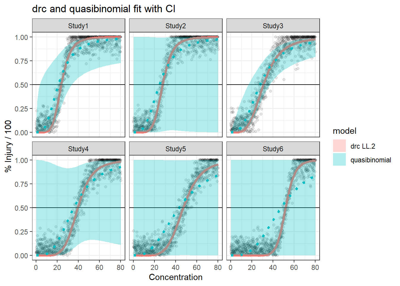
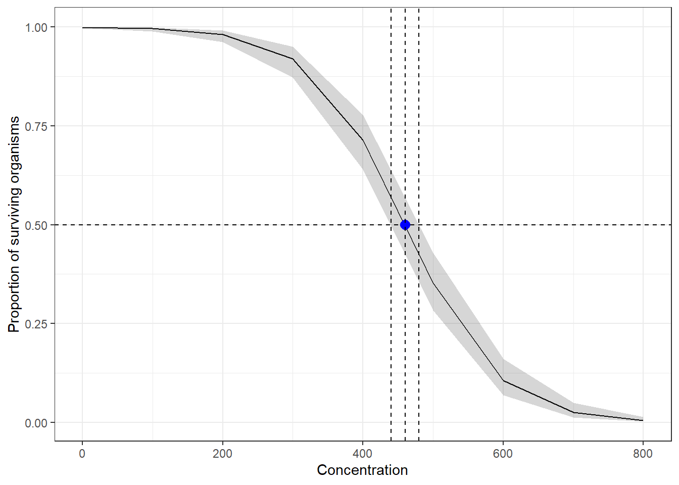
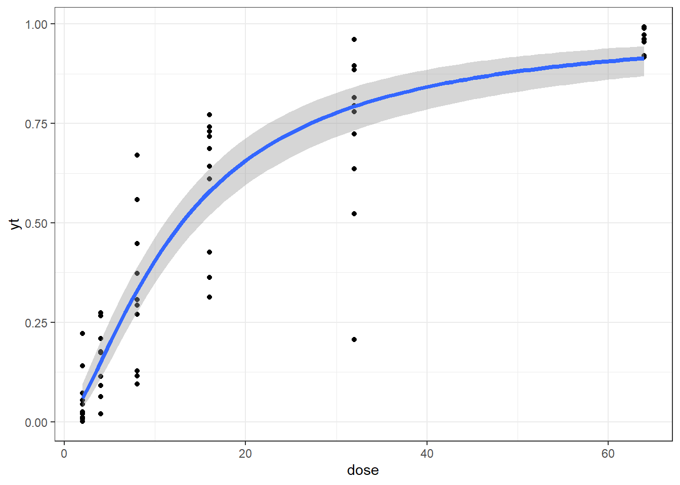
In summary, the dose reponse model with normal error predicts the true EC50 better and have smaller CI with lots of data available. We will further check the results when there are less data available.
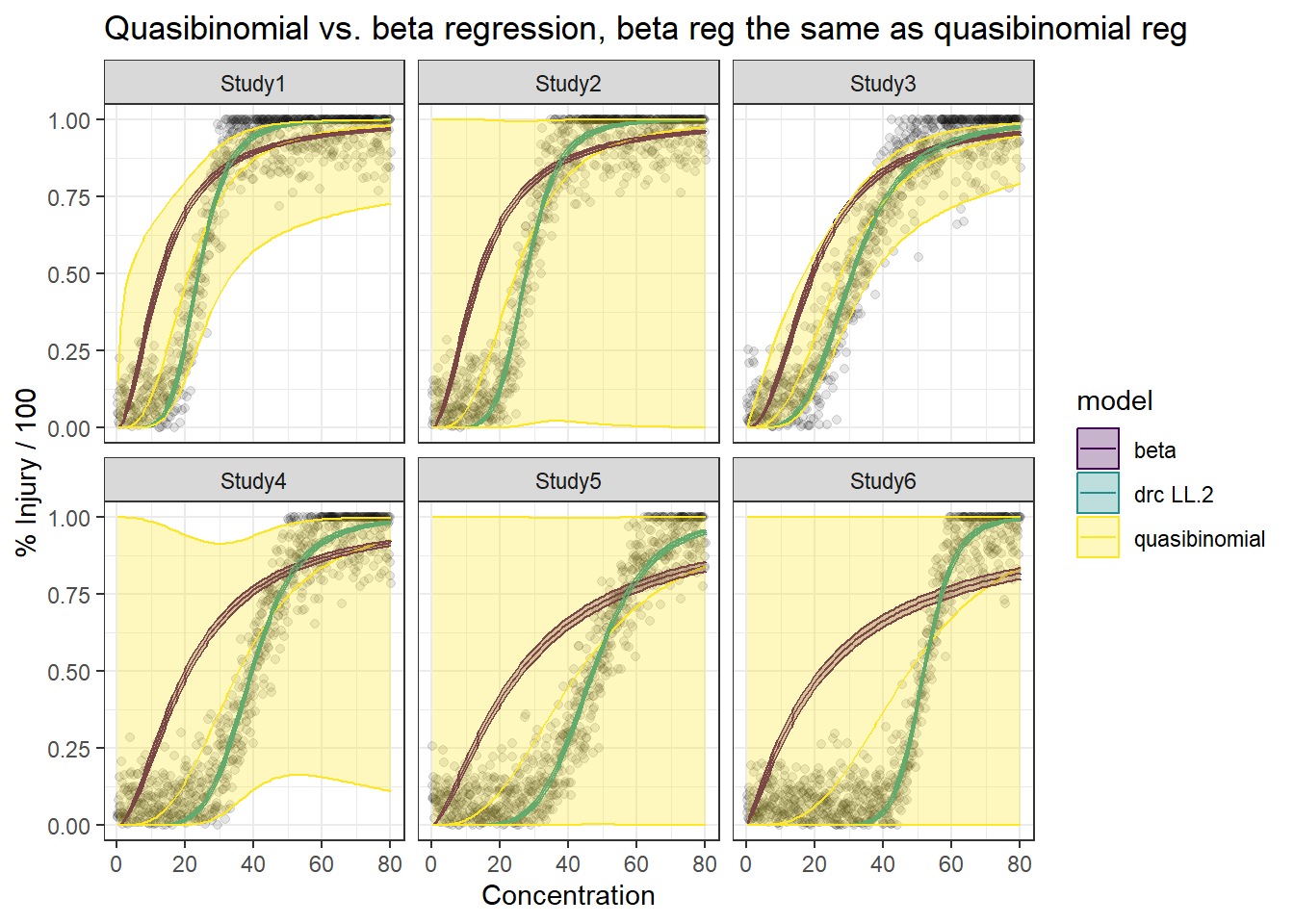
Note that the betar family in the gam package offers the same estimation as in betareg, but it can handle random effects and standard errors as well. For betareg fits, bootstrap confidence intervals need to be implemented or we need to use betareg(…, method = “BR”).
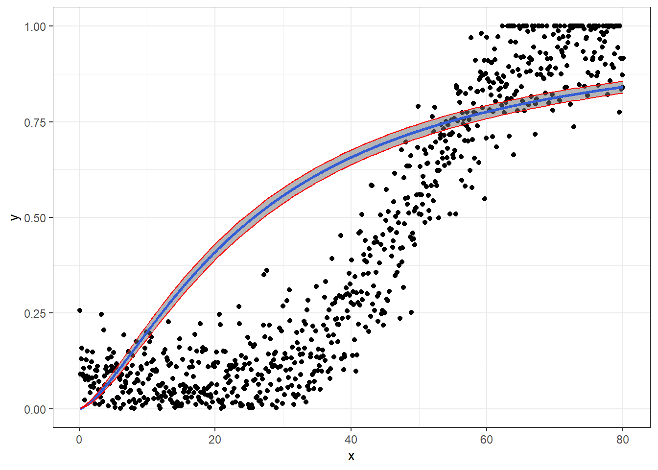
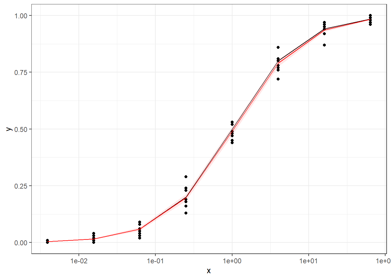
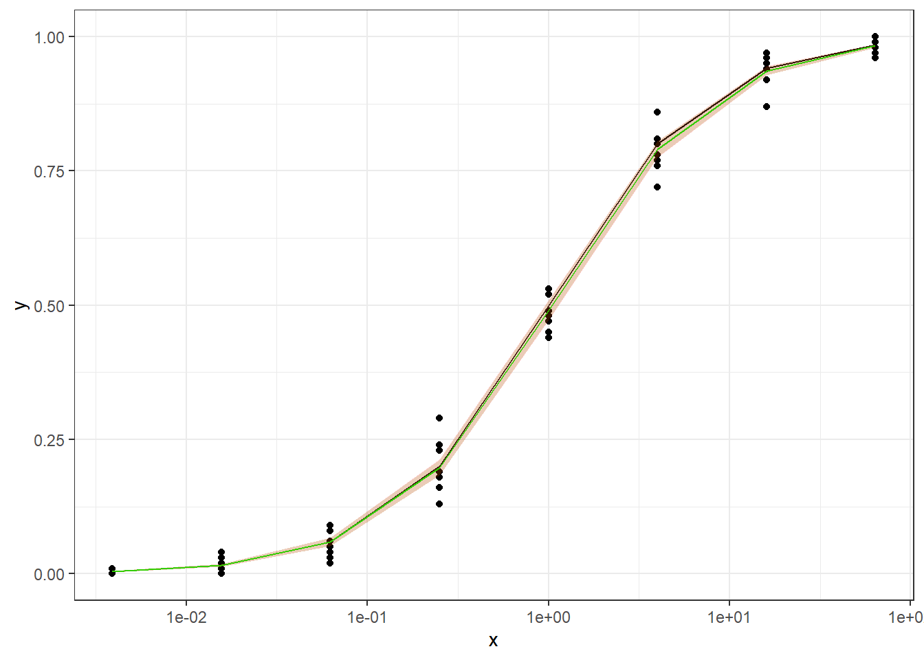
library(gam)library(mgcv)## df_all <- df_all %>% mutate(logx=log(x))mygam =gam(y ~log(x), family=betar(link="logit"), data = df_all %>%filter(study=="Study5"))min <-min(df_all$x)max <-max(df_all$x)new.x <- (expand.grid(x =seq(min, max, length.out =1000)))#new.x$logx=log(new.x$x)new.y <-predict(mygam, newdata = new.x, se.fit =TRUE, type="response")new.y <-data.frame(new.y)addThese <-data.frame(new.x, new.y)addThese <-rename(addThese, y = fit, SE = se.fit)addThese <-mutate(addThese, lwr = y -1.96* SE, upr = y +1.96* SE) # calculating the 95% confidence intervalpredbeta <-predictCIglm(mygam,dat=df_all %>%filter(study=="Study5"))ggplot(df_all%>%filter(study=="Study5"), aes(x = x, y = y)) +geom_point() +geom_smooth(data = addThese, aes(ymin = lwr, ymax = upr), stat ='identity') +geom_ribbon(data=predbeta, aes(x=x,ymin=Lower,ymax=Upper,y=Prediction),alpha=0.2,col="red")
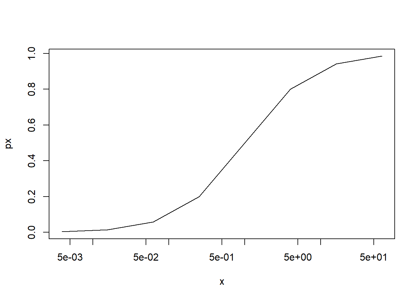
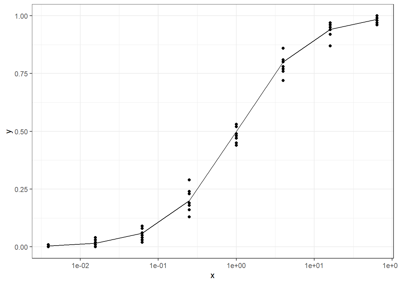
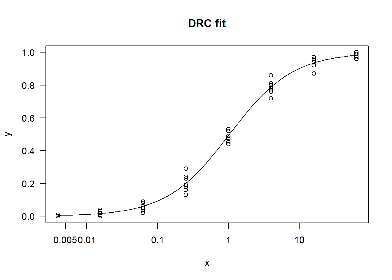
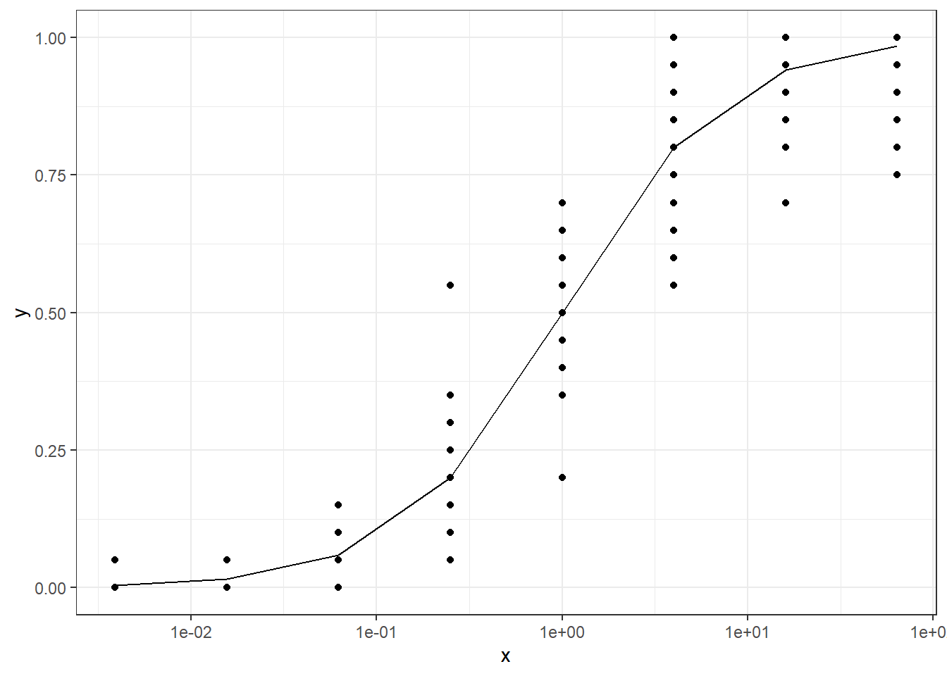
simbinomdata <- purrr::map_dfr(lapply(1:length(x),function(i,n=10,size=100){ pi <- px[i] x1 <-rep(x[i],n) yi <-rbinom(n=n,size=size,prob=pi)/sizereturn(data.frame(x=x1,y=yi))}),as.list)ggplot(simbinomdata,aes(x=x,y=y))+geom_point()+scale_x_log10()+geom_line(data=data.frame(x=x,y=px),aes(x=x,y=px))
Call:
glm(formula = y ~ log(x), family = "quasibinomial", data = simbinomdata)

Coefficients:
            Estimate Std. Error t value Pr(>|t|)
(Intercept) -0.03479    0.03518  -0.989    0.326
log(x)       0.98320    0.02022  48.618   <2e-16 ***
---
Signif. codes:  0 '***' 0.001 '**' 0.01 '*' 0.05 '.' 0.1 ' ' 1

(Dispersion parameter for quasibinomial family taken to be 0.008989206)

    Null deviance: 63.0622  on 79  degrees of freedom
Residual deviance:  0.7379  on 78  degrees of freedom
AIC: NA

Number of Fisher Scoring iterations: 6
The quasi-binomial isn’t necessarily a particular distribution. The only assumption is that for a generalized linear model with binomial assumption of “p” (mean of the binomial should be \(np\)), the variance is \(\phi\) times the variance for that binomial = np(1-p). In case of missing sample size, then it is just \(\phi p(1-p)\)
Quasi-binomial is exactly the same as binomial for the coefficient / parameter estimates but not for the standard errors. In fact, quasi-likelihood models do a post-fitting adjustment to the standard errors of the parameters and the associated statistics; they don’t change anything about the way the model is fitted. Some analysis uses observation-level random effects (OLRE) rather than quasi-likelihood to handle overdispersion at the level of individual observations. The way to adjust the coefficient standard error and to model OLRE is in this link
In terms of GLM, the dispersion for non-over-dispersed model like binomial and Poisson is 1. For quasi-families, it is estimated by the residual Chi-squared statistic divided by the residual degrees of freedom. Quasi binomial takes sqrt(overdispersion) (\(\sqrt{\Phi}\)) parameter to adjust standard errors accordingly. In case we have binomial data, the dispersion parameter can be calculated via \(\Phi = \chi^2/(N-k)\) where \(df = N-k\)
For estimation of EC50 or other ECx, other than inverse regression methods such as here and here
There is a {dose.p} function in the MASS package for calculating LCx or ECx together with the standard errors which can be used for the response confidence intervals. The vcov function can be used to extract the covariance function and used for estimation the CI of LCx or ECx. An alternative approach is to use bootstrap confidence intervals.
Since the goal of the data analysis is to measure the association between a set of regression parameters and the outcome, quasibinomial models can be useful with the variance assumption being relaxed. However, it is required to estimate the uncertainty associated with that relationship.
In fact, a limitation of these models is that they cannot yield accurate prediction intervals, the Pearson residuals cannot tell you much about how accurate the mean model is, and information criteria like the AIC or BIC cannot effectively compare these models to other types of models.
AIC(mod0)
[1] 19.40066
# [1] 19.40066try(AIC(mod1))
[1] NA
# > AIC(mod1)# Error in h(simpleError(msg, call)) :# error in evaluating the argument 'object' in selecting a method for function 'AIC': object 'mod1' not found
Generate data
logit_scale =seq(-6, 6, by =0.1)plot( logit_scale,plogis(logit_scale), ylab ='probabilities', type ='n',main="Logistic Function")lines( logit_scale,plogis(logit_scale))
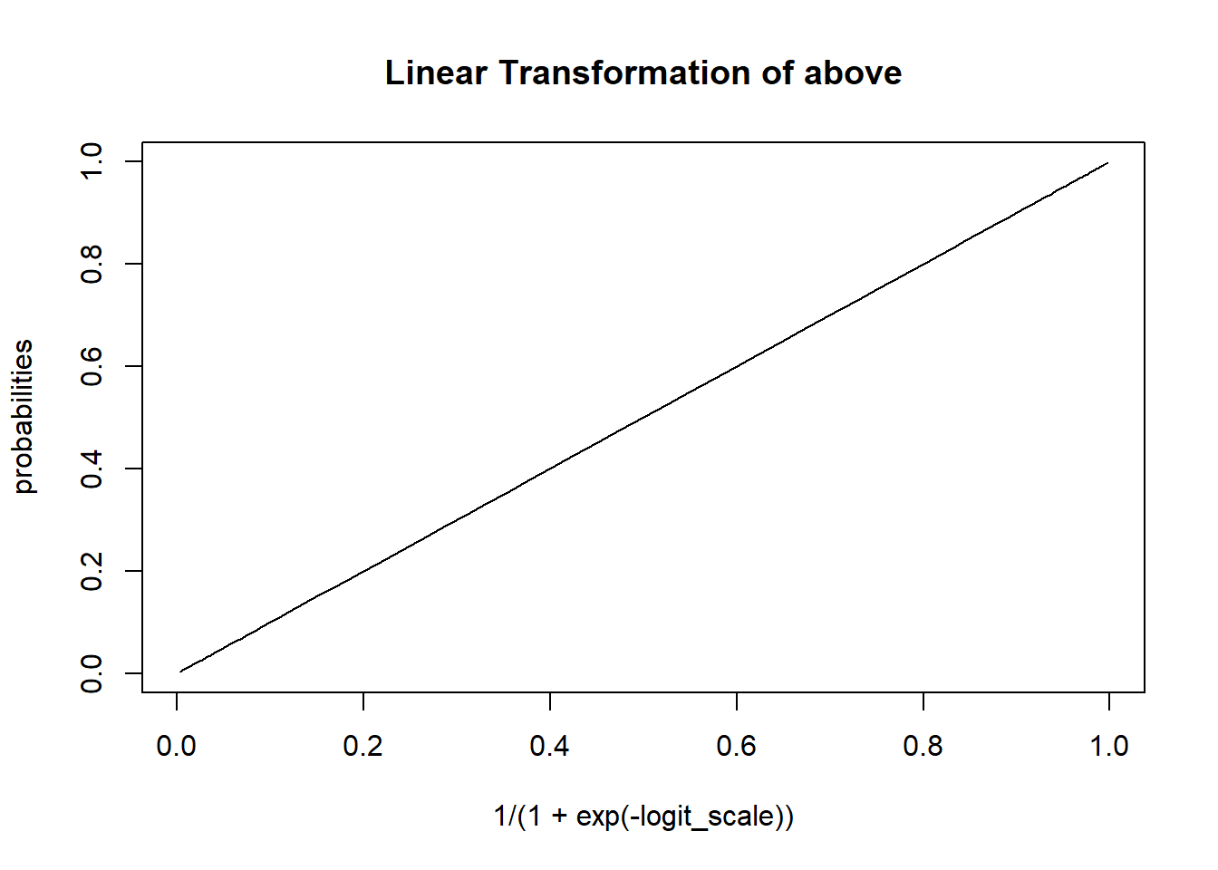
plot( 1/(1+exp(-logit_scale)),plogis(logit_scale), ylab ='probabilities', type ='l',main="Linear Transformation of above")
## fit ordered logit model and store results 'm'dattab_new $y0 <-factor(dattab_new$y0, levels =c("0","A","B","C","D","E","F"),ordered =TRUE)m <- MASS::polr(y0 ~log(dose), data = dattab_new, Hess=TRUE)summary(m)
Call:
MASS::polr(formula = y0 ~ log(dose), data = dattab_new, Hess = TRUE)

Coefficients:
          Value Std. Error t value
log(dose) 3.465     0.4876   7.106

Intercepts:
    Value   Std. Error t value
0|A  4.0061  0.8091     4.9513
A|B  6.3415  1.0283     6.1669
B|C  8.1921  1.2395     6.6092
C|D  9.1287  1.3489     6.7677
D|E 10.9709  1.5691     6.9917
E|F 12.9482  1.8234     7.1011

Residual Deviance: 128.7906
AIC: 142.7906
ctable <-coef(summary(m))## At ER50, the cumulative probability probability of the response being in a higher category is close to 1.plogis(ctable[,1] + ctable[,2]*log(12.18))
Linear mixed-effects model fit by maximum likelihood
  Data: dattab
  AIC BIC logLik
   NA  NA     NA

Random effects:
 Formula: ~1 | Obs
        (Intercept)    Residual
StdDev:   0.8883142 2.02464e-05

Variance function:
 Structure: fixed weights
 Formula: ~invwt
Fixed effects:  yt ~ log(dose)
                Value  Std.Error DF   t-value p-value
(Intercept) -4.326393 0.26598326 58 -16.26566       0
log(dose)    1.714092 0.09853347 58  17.39603       0
 Correlation:
          (Intr)
log(dose) -0.899

Standardized Within-Group Residuals:
          Min            Q1           Med            Q3           Max
-1.754784e-04 -4.189350e-05  8.955260e-06  4.092003e-05  1.439488e-04

Number of Observations: 60
Number of Groups: 60