Categorical Responses

code

analysis

Try the GLMcat package and drmOrdinal

Author

Zhenglei Gao

Published

January 10, 2025

GLMcat is an R package that encompasses lots of models specified in a similar way: (ratio, cdf, design: parallel or complete).

ratio can be cumulative, sequential, or adjacent for ordinal data, reference for nominal data. Logistic, normal, Cauchy, Student, Gompertz and Gumbel are the commonly used link functions or CDF. Note that Gumbel cdf is the symmetric of the Gompertz cdf.

For parallel design, the effects of the covariates are assumed to be constant across the response categories, whereas for complete design, the covariates effects are different across different response categories. The linear predictios are \(\eta_j=\alpha_j+x'\delta_j\) and \(\eta_j=\alpha_j+x'\delta\) for \(j\) in \((1,...,J-1)\)

There are several type of models for categorical data:

multinomial (reference, logistic, complete) –> devoted to nominal instead of ordinal
odds parallel logit (cumulative, logistic, parallel)
parallel hazard (sequential, gompertz, parallel)
continuation ratio logit model (sequential, logistic, complete)
adjacent logit model (adjacent, logistic, complete)

Code

library(tidyverse)

The dataset used in a previous post

The data was generated by Changjian using SAS Probnorm with Vx=0.25 and Vr=0.15, a=-2.5, b=1.0, ER50=12.18. Model: probit(y) = a + b*logdose + ri;

Code

pnorm(-2.5+1*log(c(2L, 4L, 8L,16L, 32L,  64L)))

[1] 0.03539262 0.13270274 0.33703877 0.60741531 0.83291183 0.95143032

Code

dattab_new <- read.table(textConnection("Obs    rep dose    yt  y0 
1   1   2   0.02021 0
2   2   2   0.02491 0
3   3   2   0.00760 0
4   5   2   0.04466 0
5   6   2   0.00037 0
6   8   2   0.05386 0
7   9   2   0.07205 0
8   10  2   0.01125 0
9   1   4   0.02011 0
10  7   4   0.09058 0
11  8   4   0.06255 0
12  10  8   0.09431 0
13  4   2   0.14060 A
14  7   2   0.22223 A
15  2   4   0.20943 A
16  3   4   0.20959 A
17  4   4   0.17305 A
18  9   4   0.11405 A
19  10  4   0.17668 A
20  1   8   0.12756 A
21  6   8   0.11478 A
22  6   32  0.20602 A
23  5   4   0.26650 B
24  6   4   0.27344 B
25  3   8   0.27021 B
26  5   8   0.30662 B
27  8   8   0.29319 B
28  9   8   0.37300 B
29  6   16  0.36224 B
30  9   16  0.31316 B
31  2   8   0.55845 C
32  4   8   0.44811 C
33  3   16  0.42677 C
34  3   32  0.52315 C
35  7   8   0.67080 D
36  2   16  0.71776 D
37  4   16  0.73038 D
38  5   16  0.64232 D
39  7   16  0.68720 D
40  8   16  0.61088 D
41  5   32  0.72342 D
42  8   32  0.63594 D
43  1   16  0.77171 E
44  10  16  0.74087 E
45  2   32  0.79477 E
46  4   32  0.88546 E
47  7   32  0.78002 E
48  9   32  0.81456 E
49  10  32  0.89465 E
50  1   32  0.96129 F
51  1   64  0.96127 F
52  2   64  0.91687 F
53  3   64  0.97204 F
54  4   64  0.99268 F
55  5   64  0.98935 F
56  6   64  0.96263 F
57  7   64  0.95435 F
58  8   64  0.92081 F
59  9   64  0.91776 F
60  10  64  0.99104 F"),header = TRUE)

Code

dattab_new <- dattab_new %>% mutate(yy = as.numeric(plyr::mapvalues(y0,from = c("0","A","B","C","D","E","F"),to = c(0,10,30,50,70,90,100)))/100) %>% mutate(yy2 = as.numeric(plyr::mapvalues(y0,from = c("0","A","B","C","D","E","F"),to = c(0.05,0.18,0.34,0.50,0.66,0.82,0.95))))

ftable(xtabs(~ y0 + dose, data = dattab_new)) ##%>% gt::gt() ## as.data.frame(.) %>% knitr::kable(.,digits = 3)

   dose  2  4  8 16 32 64
y0                       
0        8  3  1  0  0  0
A        2  5  2  0  1  0
B        0  2  4  2  0  0
C        0  0  2  1  1  0
D        0  0  1  5  2  0
E        0  0  0  2  5  0
F        0  0  0  0  1 10

Code

dattab_new %>% group_by(y0) %>% summarise(n=n(),meany=mean(yt),meanyy2=mean(yy2)) %>% knitr::kable(.,digits = 3)

y0	n	meany	meanyy2
0	12	0.042	0.05
A	10	0.169	0.18
B	8	0.307	0.34
C	4	0.489	0.50
D	8	0.677	0.66
E	7	0.812	0.82
F	11	0.958	0.95

Code

dattab_new %>% group_by(dose) %>% summarise(n=n(),meany=mean(yt),meanyy=mean(yy)) %>% knitr::kable(.,digits = 3)

dose	n	meany	meanyy
2	10	0.060	0.02
4	10	0.160	0.11
8	10	0.326	0.31
16	10	0.600	0.64
32	10	0.722	0.75
64	10	0.958	1.00

Code

ggplot(dattab_new,aes(x = dose, y=yt))+geom_point() +  geom_smooth(method="glm", method.args=list(family="quasibinomial"), formula="y ~ log(x)",
                       se =TRUE, size=1.5)

Warning: Using `size` aesthetic for lines was deprecated in ggplot2 3.4.0.
ℹ Please use `linewidth` instead.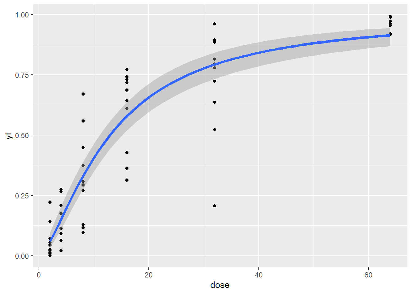

y0	2	4	8	16	32	64
0	8	3	1	0	0	0
A	2	5	2	0	1	0
B	0	2	4	2	0	0
C	0	0	2	1	1	0
D	0	0	1	5	2	0
E	0	0	0	2	5	0
F	0	0	0	0	1	10

Code

## fit ordered logit model and store results 'm'
dattab_new $y0 <- factor(dattab_new$y0, levels = c("0","A","B","C","D","E","F"),ordered = TRUE)

m <- MASS::polr(y0 ~ log(dose), data = dattab_new, Hess=TRUE)
summary(m)

Call:
MASS::polr(formula = y0 ~ log(dose), data = dattab_new, Hess = TRUE)

Coefficients:
          Value Std. Error t value
log(dose) 3.465     0.4876   7.106

Intercepts:
    Value   Std. Error t value
0|A  4.0061  0.8091     4.9513
A|B  6.3415  1.0283     6.1669
B|C  8.1921  1.2395     6.6092
C|D  9.1287  1.3489     6.7677
D|E 10.9709  1.5691     6.9917
E|F 12.9482  1.8234     7.1011

Residual Deviance: 128.7906 
AIC: 142.7906

Code

ctable <- coef(summary(m))

## At ER50, the cumulative probability probability of the response being in a higher category is close to 1.
plogis(ctable[,1] + ctable[,2]*log(12.18))

log(dose)       0|A       A|B       B|C       C|D       D|E       E|F 
0.9908438 0.9975973 0.9998653 0.9999875 0.9999963 0.9999997 1.0000000

Code

## calculate and store p values
p <- pnorm(abs(ctable[, "t value"]), lower.tail = FALSE) * 2

## combined table
(ctable <- cbind(ctable, "p value" = p))

              Value Std. Error  t value      p value
log(dose)  3.465155  0.4876298 7.106117 1.193530e-12
0|A        4.006148  0.8091031 4.951344 7.370254e-07
A|B        6.341529  1.0283150 6.166913 6.963590e-10
B|C        8.192141  1.2395138 6.609156 3.865169e-11
C|D        9.128696  1.3488680 6.767672 1.308710e-11
D|E       10.970866  1.5691374 6.991654 2.716642e-12
E|F       12.948174  1.8234117 7.101070 1.237950e-12

Code

(ci <- confint(m)) ## profiled CI

Waiting for profiling to be done...

   2.5 %   97.5 % 
2.582836 4.504378

Code

exp(cbind(coef(m),t(ci)))

                      2.5 %   97.5 %
log(dose) 31.98141 13.23462 90.41212

Code

## OR and CI
exp(cbind(OR = coef(m), ci))

             OR       ci
2.5 %  31.98141 13.23462
97.5 % 31.98141 90.41212

Code

newdat <- data.frame(dose = unique(dattab_new$dose)) %>% mutate(logdose = log(dose))
(phat <- predict(object = m, newdat, type="p"))

             0            A           B           C          D            E
1 8.326166e-01 0.1483000019 0.016035611 0.001850927 0.00100702 0.0001635762
2 3.105443e-01 0.5126011687 0.144195119 0.019598385 0.01096824 0.0018025754
3 3.918687e-02 0.2573055374 0.431914336 0.144078094 0.10487831 0.0194406374
4 3.342916e-04 0.0031093320 0.018073161 0.031603441 0.20832988 0.4574198047
5 3.679470e-03 0.0330795765 0.158639125 0.187148646 0.41376767 0.1694853156
6 3.027903e-05 0.0002825179 0.001674417 0.003066947 0.02600507 0.1569497884
             F
1 2.628958e-05
2 2.902582e-04
3 3.196213e-03
4 2.811301e-01
5 3.420020e-02
6 8.119910e-01

Code

phat %>% knitr::kable(.,digits = 3)

0	A	B	C	D	E	F
0.833	0.148	0.016	0.002	0.001	0.000	0.000
0.311	0.513	0.144	0.020	0.011	0.002	0.000
0.039	0.257	0.432	0.144	0.105	0.019	0.003
0.000	0.003	0.018	0.032	0.208	0.457	0.281
0.004	0.033	0.159	0.187	0.414	0.169	0.034
0.000	0.000	0.002	0.003	0.026	0.157	0.812

Code

library(GLMcat)

Warning: package 'GLMcat' was built under R version 4.4.2

Code

dattab_new <- dattab_new %>% mutate(logdose = log(dose))
mod_ref_log_c <- glmcat(formula = y0 ~ logdose, ratio = "reference", cdf = "logistic", data = as.data.frame(dattab_new),ref="0",parallel = F)

Warning in glmcat(formula = y0 ~ logdose, ratio = "reference", cdf =
"logistic", : The response variable is defined as an ordered variable. Recall
that the the reference ratio is appropiate for nominal responses, while for
ordinal responses the ratios to use are cumulative, sequential or adjacent.

Code

summary(mod_ref_log_c)

y0 ~ logdose
                ratio      cdf nobs niter    logLik
Model info: reference logistic   60    15 -61.33542
                Estimate Std. Error z value Pr(>|z|)    
(Intercept) A     -2.907      1.309  -2.221 0.026323 *  
(Intercept) B     -5.398      1.835  -2.942 0.003260 ** 
(Intercept) C     -9.347      3.019  -3.096 0.001958 ** 
(Intercept) D    -10.923      3.065  -3.564 0.000366 ***
(Intercept) E    -17.421      4.838  -3.600 0.000318 ***
(Intercept) F   -118.572 109742.484  -0.001 0.999138    
logdose A          2.179      0.993   2.194 0.028225 *  
logdose B          3.415      1.177   2.901 0.003725 ** 
logdose C          4.803      1.504   3.194 0.001404 ** 
logdose D          5.633      1.499   3.758 0.000172 ***
logdose E          7.692      1.895   4.058 4.94e-05 ***
logdose F         36.404  31664.987   0.001 0.999083    
---
Signif. codes:  0 '***' 0.001 '**' 0.01 '*' 0.05 '.' 0.1 ' ' 1

Code

(phat <- predict(object = mod_ref_log_c, newdat, type="prob"))

                A            B            C            D            E
[1,] 1.904456e-01 3.716346e-02 1.873707e-03 6.891895e-04 4.324730e-06
[2,] 4.075170e-01 1.873256e-01 2.472185e-02 1.616443e-02 4.225492e-04
[3,] 3.188563e-01 3.452649e-01 1.192710e-01 1.386298e-01 1.509628e-02
[4,] 5.226961e-03 3.140645e-02 7.433584e-02 2.730262e-01 5.159543e-01
[5,] 7.795418e-02 1.988396e-01 1.797976e-01 3.714905e-01 1.685225e-01
[6,] 2.602306e-12 3.683274e-11 2.281981e-10 1.489911e-09 1.172908e-08
                F            0
[1,] 2.238505e-41 7.698238e-01
[2,] 9.621081e-31 3.638486e-01
[3,] 1.512043e-20 6.288173e-02
[4,] 1.000000e-01 5.029071e-05
[5,] 7.425049e-11 3.395654e-03
[6,] 1.000000e+00 5.551115e-15

Code

phat %>% knitr::kable(.,digits = 3)

A	B	C	D	E	F	0
0.190	0.037	0.002	0.001	0.000	0.0	0.770
0.408	0.187	0.025	0.016	0.000	0.0	0.364
0.319	0.345	0.119	0.139	0.015	0.0	0.063
0.005	0.031	0.074	0.273	0.516	0.1	0.000
0.078	0.199	0.180	0.371	0.169	0.0	0.003
0.000	0.000	0.000	0.000	0.000	1.0	0.000

Code

## (phat <- predict(object = mod_ref_log_c, newdat, type="linear.predictor"))

mod_cum_logis <- glmcat(formula = y0 ~ logdose, ratio = "cumulative", cdf = "logistic", data = as.data.frame(dattab_new),parallel = TRUE)
summary(mod_cum_logis)

y0 ~ logdose
                 ratio      cdf nobs niter   logLik
Model info: cumulative logistic   60     9 -64.3953
              Estimate Std. Error z value Pr(>|z|)    
(Intercept) 0   4.0061     0.8142   4.920 8.64e-07 ***
(Intercept) A   6.3415     1.0419   6.086 1.16e-09 ***
(Intercept) B   8.1920     1.2583   6.510 7.50e-11 ***
(Intercept) C   9.1286     1.3693   6.666 2.62e-11 ***
(Intercept) D  10.9707     1.6005   6.854 7.16e-12 ***
(Intercept) E  12.9479     1.8194   7.117 1.11e-12 ***
logdose        -3.4651     0.4912  -7.054 1.74e-12 ***
---
Signif. codes:  0 '***' 0.001 '**' 0.01 '*' 0.05 '.' 0.1 ' ' 1

Code

(phat <- predict(object = mod_cum_logis, newdat, type="prob"))

                0            A           B           C           D           E
[1,] 8.326186e-01 0.1482975531 0.016035767 0.001851046 0.001007102 0.000163596
[2,] 3.105557e-01 0.5125923926 0.144191357 0.019598856 0.010968693 0.001802725
[3,] 3.919032e-02 0.2573138937 0.431903119 0.144076171 0.104878455 0.019441472
[4,] 3.343480e-04 0.0031097342 0.018074387 0.031605029 0.208331116 0.457408504
[5,] 3.679947e-03 0.0330824671 0.158642283 0.187148395 0.413758936 0.169485389
[6,] 3.028531e-05 0.0002825654 0.001674598 0.003067232 0.026006412 0.156948672
                F
[1,] 2.629451e-05
[2,] 2.903015e-04
[3,] 3.196565e-03
[4,] 2.811369e-01
[5,] 3.420258e-02
[6,] 8.119902e-01

Code

phat %>% knitr::kable(.,digits = 3)

0	A	B	C	D	E	F
0.833	0.148	0.016	0.002	0.001	0.000	0.000
0.311	0.513	0.144	0.020	0.011	0.002	0.000
0.039	0.257	0.432	0.144	0.105	0.019	0.003
0.000	0.003	0.018	0.032	0.208	0.457	0.281
0.004	0.033	0.159	0.187	0.414	0.169	0.034
0.000	0.000	0.002	0.003	0.026	0.157	0.812

Other understanding of the dataset

Code

fit0 <- MASS::polr(y0 ~ 1,
                      data = dattab_new,
                      Hess= T)
fit0

Call:
MASS::polr(formula = y0 ~ 1, data = dattab_new, Hess = T)

No coefficients

Intercepts:
          0|A           A|B           B|C           C|D           D|E 
-1.386294e+00 -5.465462e-01 -1.793225e-06  2.682586e-01  8.472940e-01 
          E|F 
 1.493920e+00 

Residual Deviance: 228.003 
AIC: 240.003

Code

#source("https://github.com/rwnahhas/RMPH_Resources/raw/main/Functions_rmph.R")
ilogit <- function(x) exp(x)/(1+exp(x))
ilogit(fit0$zeta)

      0|A       A|B       B|C       C|D       D|E       E|F 
0.2000001 0.3666661 0.4999996 0.5666653 0.6999992 0.8166659

Code

sf <- function(y) {
  c('Y>=1' = qlogis(mean(y >= 1)),
    'Y>=2' = qlogis(mean(y >= 2)),
    'Y>=3' = qlogis(mean(y >= 3)),
    'Y>=4' = qlogis(mean(y >= 4)),
    'Y>=5' = qlogis(mean(y >= 5)))
}

(s <- with(dattab_new, summary(as.numeric(y0) ~ factor(dose), fun=sf)))

 Length   Class    Mode 
      3 formula    call

Code

glm(I(as.numeric(y0) >= 2) ~ log(dose), family="binomial", data = dattab_new)


Call:  glm(formula = I(as.numeric(y0) >= 2) ~ log(dose), family = "binomial", 
    data = dattab_new)

Coefficients:
(Intercept)    log(dose)  
     -3.305        2.874  

Degrees of Freedom: 59 Total (i.e. Null);  58 Residual
Null Deviance:      60.05 
Residual Deviance: 29.19    AIC: 33.19

Code

glm(I(as.numeric(y0) >= 3) ~ log(dose), family="binomial", data = dattab_new)


Call:  glm(formula = I(as.numeric(y0) >= 3) ~ log(dose), family = "binomial", 
    data = dattab_new)

Coefficients:
(Intercept)    log(dose)  
     -5.089        2.726  

Degrees of Freedom: 59 Total (i.e. Null);  58 Residual
Null Deviance:      78.86 
Residual Deviance: 33.83    AIC: 37.83

Code

glm(I(as.numeric(y0) >= 4) ~ log(dose), family="binomial", data = dattab_new)


Call:  glm(formula = I(as.numeric(y0) >= 4) ~ log(dose), family = "binomial", 
    data = dattab_new)

Coefficients:
(Intercept)    log(dose)  
     -7.440        3.067  

Degrees of Freedom: 59 Total (i.e. Null);  58 Residual
Null Deviance:      83.18 
Residual Deviance: 30.69    AIC: 34.69

log-logistic with quasi-binomial

TRUE ER50=12.18.

Code

getEC50 <- function(mod){
  if("glm" %in% class(mod)){
    ec50 <- MASS::dose.p(mod,p=0.5)
    se <- attr(ec50,"SE")
    xmin <- as.numeric(ec50 - 1.96*se)
    xmax <- as.numeric(ec50 + 1.96*se) 
    res <- data.frame(EC50=exp(as.numeric(ec50)),
    lower=exp(xmin),upper=exp(xmax),se=se)
  }else{
    if("glmmPQL" %in% class(mod)){
      res1 <- dose.p.glmmPQL(mod,cf=1:2,p=0.5)
      se <- attr(res1,"SE")
      res <- data.frame(EC50=exp(res1[1]),lower=exp(res1[1]-1.96*se),upper=exp(res1[1]+1.96*se),se=se)
    }else{
      res1 <- ED(mod,50,interval="delta")
      res <- data.frame(EC50=res1[1,"Estimate"],lower=res1[1,"Lower"],upper=res1[1,"Upper"],se=res1[1,"Std. Error"])

    }
  }
  return(res)
}

dose.p.glmmPQL <- function(obj,cf=1:2,p=0.5){
  eta <- obj$family$linkfun(p)
  b <- obj$coefficients$fixed[cf]
  x.p <- (eta - b[1L])/b[2L]
  names(x.p) <- paste("p = ", format(p), ":", sep = "")
  pd <- -cbind(1, x.p)/b[2L]
  SE <- sqrt(((pd %*% vcov(obj)[cf, cf]) * pd) %*% c(1, 1))
  res <- structure(x.p, SE = SE, p = p)
  class(res) <- "glm.dose"
  res
}

Code

mod <- glm(yy2~log(dose),data = dattab_new,family = quasibinomial)
summary(mod)


Call:
glm(formula = yy2 ~ log(dose), family = quasibinomial, data = dattab_new)

Coefficients:
            Estimate Std. Error t value Pr(>|t|)    
(Intercept)  -3.5064     0.3132  -11.19 4.02e-16 ***
log(dose)     1.3832     0.1171   11.81  < 2e-16 ***
---
Signif. codes:  0 '***' 0.001 '**' 0.01 '*' 0.05 '.' 0.1 ' ' 1

(Dispersion parameter for quasibinomial family taken to be 0.1163524)

    Null deviance: 31.8277  on 59  degrees of freedom
Residual deviance:  6.3595  on 58  degrees of freedom
AIC: NA

Number of Fisher Scoring iterations: 5

Code

ER50 <- exp(-coef(mod)[1]/coef(mod)[2])
ER50

(Intercept) 
     12.617

Code

getEC50(mod)

           EC50    lower    upper         se
p = 0.5: 12.617 10.77038 14.78023 0.08073738

Code

pred <- predict(mod,newdata = dattab_new,type = "response")
dattab_new$pred <- pred
dattab_new %>% group_by(y0) %>% summarise(n=n(),meany=mean(yt),meanyy2=mean(yy2),meanEst=mean(pred)) %>% knitr::kable(.,digits = 3)

y0	n	meany	meanyy2	meanEst
0	12	0.042	0.05	0.120
A	10	0.169	0.18	0.247
B	8	0.307	0.34	0.361
C	4	0.489	0.50	0.515
D	8	0.677	0.66	0.603
E	7	0.812	0.82	0.726
F	11	0.958	0.95	0.893

Code

## Consider Replicate effect
modr <- MASS::glmmPQL(yy2~ log(dose),random=~1|rep,family="quasibinomial",data=dattab_new)
ER50 <- exp(-coef(modr)[1]/coef(modr)[2])
exp(-modr$coefficients$fixed[1]/ modr$coefficients$fixed[2])

(Intercept) 
   12.61695

Code

summary(modr)

Linear mixed-effects model fit by maximum likelihood
  Data: dattab_new 
  AIC BIC logLik
   NA  NA     NA

Random effects:
 Formula: ~1 | rep
        (Intercept)  Residual
StdDev:   0.2256918 0.3155037

Variance function:
 Structure: fixed weights
 Formula: ~invwt 
Fixed effects:  yy2 ~ log(dose) 
                Value Std.Error DF   t-value p-value
(Intercept) -3.517527 0.3039553 49 -11.57251       0
log(dose)    1.387562 0.1103306 49  12.57640       0
 Correlation: 
          (Intr)
log(dose) -0.907

Standardized Within-Group Residuals:
       Min         Q1        Med         Q3        Max 
-3.9592347 -0.3047297  0.1382668  0.4944066  1.9353183 

Number of Observations: 60
Number of Groups: 10

Code

getEC50(modr)

             EC50    lower    upper         se
p = 0.5: 12.61695 10.56476 15.06777 0.09057011

Code

pred <- predict(modr,newdata = dattab_new,type = "response")
dattab_new$predr <- pred
dattab_new %>% group_by(y0) %>% summarise(n=n(),meany=mean(yt),meanyy2=mean(yy2),meanEst=mean(pred),meanEstR=mean(predr)) %>% knitr::kable(.,digits = 3)

y0	n	meany	meanyy2	meanEst	meanEstR
0	12	0.042	0.05	0.120	0.120
A	10	0.169	0.18	0.247	0.240
B	8	0.307	0.34	0.361	0.342
C	4	0.489	0.50	0.515	0.517
D	8	0.677	0.66	0.603	0.620
E	7	0.812	0.82	0.726	0.736
F	11	0.958	0.95	0.893	0.894

Note that glmer and glmmPQL (based on lme from the nlme pacakge) differs in terms of parameter estimation algorithm and nlme is not optimized for dealing with crossed random effects, which are associated with a sparse design matrix. See more in the book from Pinheiro & Bates.[^1]

Code

uniroot(function(x) {
  y <- as.numeric(predict(modr, newdata = data.frame(dose=x,rep=1),level=0) - 0.5)
  },lower =10, upper = 25)$root

[1] 18.09047

Dose Response for continuous data

Code

ggplot(dattab_new,aes(x = dose, y=yy2))+geom_point() +  geom_smooth(method="glm", method.args=list(family="quasibinomial"), formula="y ~ log(x)",
                       se =TRUE, size=1.5)+scale_x_log10() +ggtitle(paste("log-logistic + quasibinomial, ER50=",round(ER50,2)))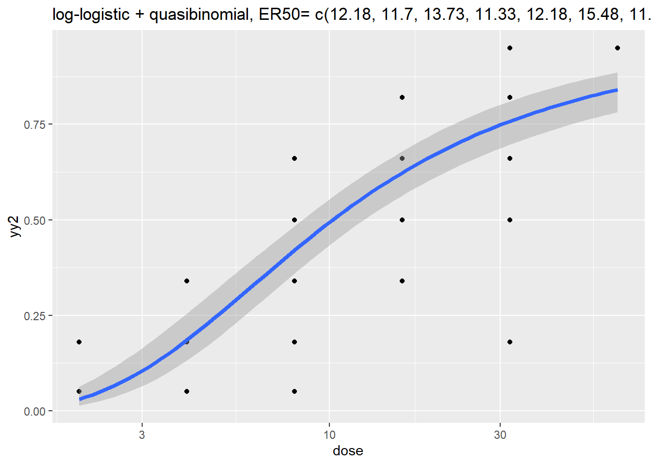

Code

library(drc)
mod_drc  <- drm(yy2 ~ dose, data = dattab_new, fct = LL.2())
## mod_drc  <- drm(yy2 ~ dose, data = dattab_new, fct = LL.2(),type = "binomial")

summary(mod_drc)


Model fitted: Log-logistic (ED50 as parameter) with lower limit at 0 and upper limit at 1 (2 parms)

Parameter estimates:

              Estimate Std. Error t-value   p-value    
b:(Intercept) -1.33865    0.13595 -9.8465 5.487e-14 ***
e:(Intercept) 12.74391    1.03919 12.2633 < 2.2e-16 ***
---
Signif. codes:  0 '***' 0.001 '**' 0.01 '*' 0.05 '.' 0.1 ' ' 1

Residual standard error:

 0.1446638 (58 degrees of freedom)

Code

ED(mod_drc, c(50), interval = "delta")


Estimated effective doses

       Estimate Std. Error   Lower   Upper
e:1:50  12.7439     1.0392 10.6637 14.8241

Code

plot(mod_drc, type = "all",main="log-logistic + normal, ER50= 12.74", broken = TRUE)
plot(mod_drc, broken = TRUE, type="confidence", add=TRUE)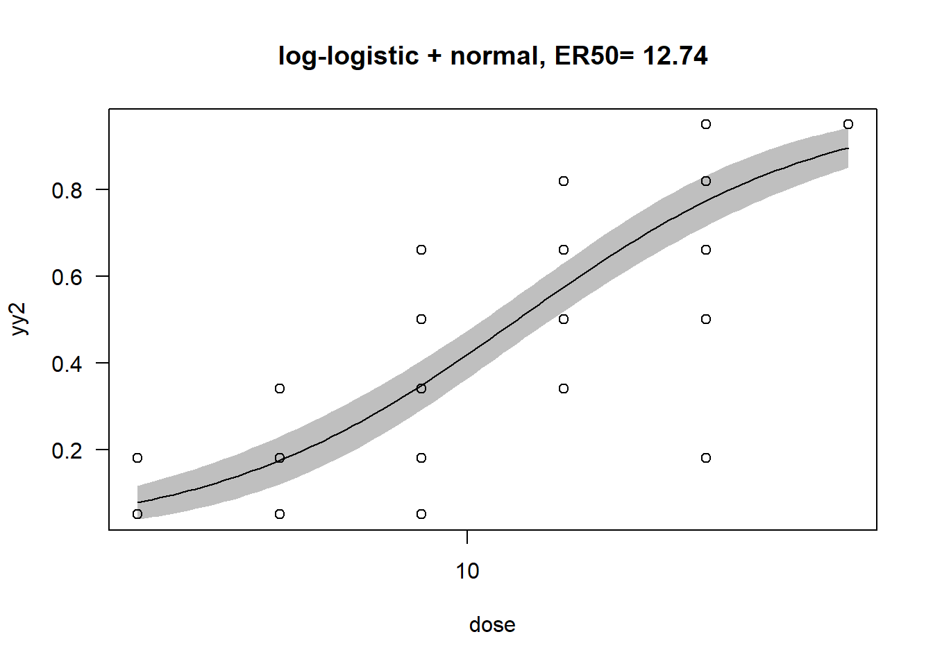

DRM Ordinal

Code

library(drc)
library(bmd)
dat_ord <- dattab_new %>% group_by(y0,dose) %>% summarise(n=n()) %>% ungroup() %>% pivot_wider(names_from = y0,values_from = n)

`summarise()` has grouped output by 'y0'. You can override using the `.groups`
argument.

Code

dat_ord <- dat_ord %>% mutate(across(c(`0`,`A`,`B`,`C`,`D`,`E`,`F`),~ifelse(is.na(.),0,.))) %>% mutate(total=rowSums(across(c(`0`,`A`,`B`,`C`,`D`,`E`,`F`))))
mod_ord <- drmOrdinal(levels = unique(dattab_new$y0),  weights="total",dose = "dose", data = dat_ord, fct = LL.2())
plot(mod_ord) # uses ggplot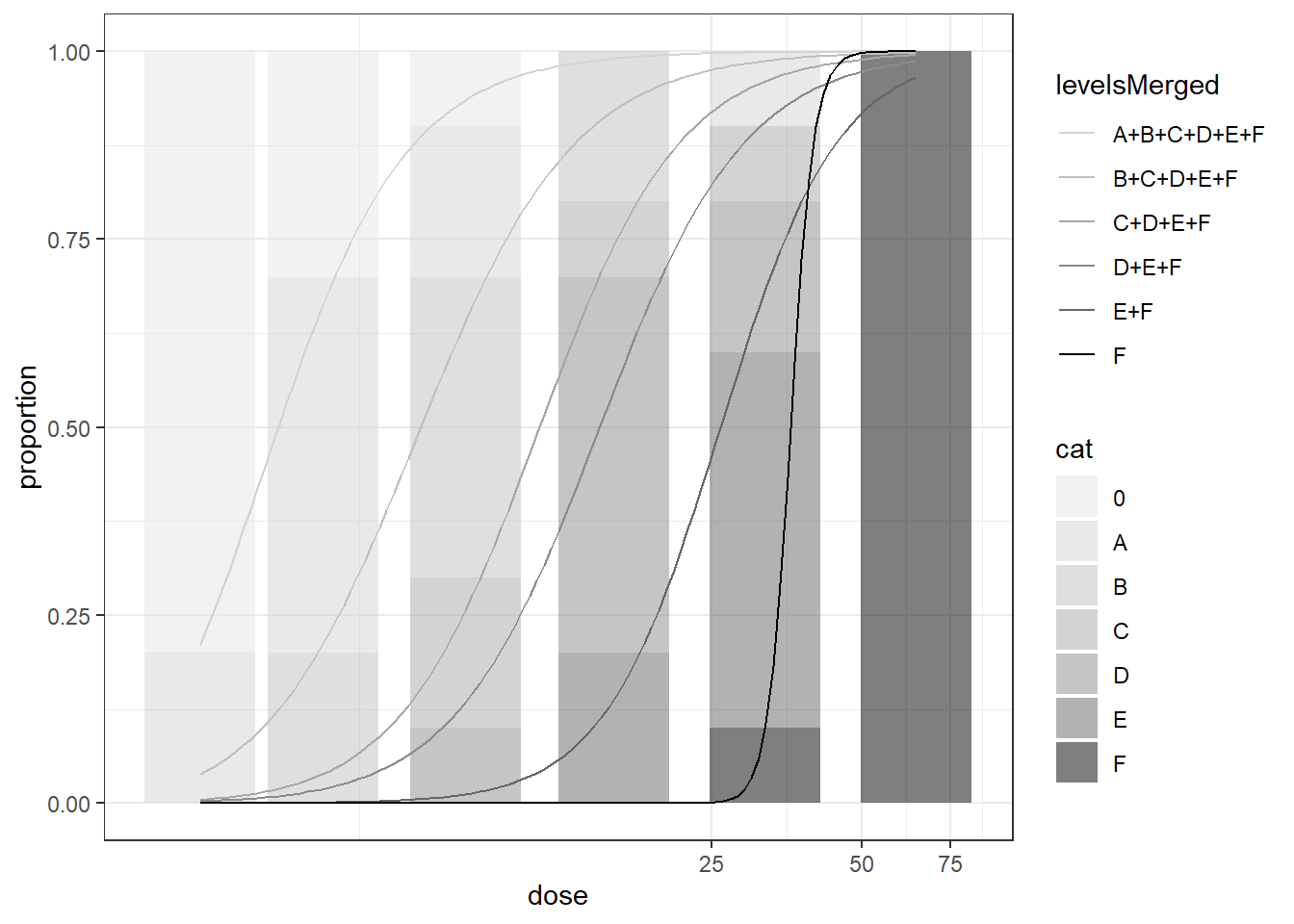

Code

bmdOrdinal(mod_ord, bmr = 0.5, backgType = "modelBased", def = "excess")

                  BMD      BMDL
A+B+C+D+E+F  3.158208  2.298134
B+C+D+E+F    6.467922  4.757317
C+D+E+F     11.313719  8.507258
D+E+F       14.947346 11.193140
E+F         26.084222 20.202286
F           35.967446 -1.757891

GLMcat Basics

Code

library(GLMcat)
data("DisturbedDreams")
summary(DisturbedDreams)

      Age                Level    
 Min.   : 6.00   Not.severe :100  
 1st Qu.: 8.50   Severe.1   : 42  
 Median :10.50   Severe.2   : 41  
 Mean   :10.96   Very.severe: 40  
 3rd Qu.:12.50                    
 Max.   :14.50

Code

head(DisturbedDreams)

  Age      Level
1   6 Not.severe
2   6 Not.severe
3   6 Not.severe
4   6 Not.severe
5   6 Not.severe
6   6 Not.severe

Code

DisturbedDreams$Level <- as.factor(as.character(DisturbedDreams$Level))
mod_ref_log_c <- glmcat(
formula = Level ~ Age, ratio = "reference",
cdf = "logistic", ref_category = "Very.severe",
data = DisturbedDreams
)

Code

summary(mod_ref_log_c)

Level ~ Age
                ratio      cdf nobs niter    logLik
Model info: reference logistic  223     5 -277.1345
                       Estimate Std. Error z value Pr(>|z|)    
(Intercept) Not.severe -2.45444    0.84559  -2.903   0.0037 ** 
(Intercept) Severe.1   -0.55464    0.89101  -0.622   0.5336    
(Intercept) Severe.2   -1.12464    0.91651  -1.227   0.2198    
Age Not.severe          0.30999    0.07804   3.972 7.13e-05 ***
Age Severe.1            0.05997    0.08582   0.699   0.4847    
Age Severe.2            0.11228    0.08684   1.293   0.1960    
---
Signif. codes:  0 '***' 0.001 '**' 0.01 '*' 0.05 '.' 0.1 ' ' 1

Code

# Random observations
set.seed(13)
ind <- sample(x = 1:nrow(DisturbedDreams), size = 3)
# Probabilities
predict(mod_ref_log_c, newdata = DisturbedDreams[ind, ], type = "prob")

     Not.severe  Severe.1  Severe.2 Very.severe
[1,]  0.5392049 0.1583321 0.1721826   0.1302804
[2,]  0.1832207 0.2732519 0.2115046   0.3320229
[3,]  0.2996414 0.2391879 0.2110034   0.2501674

Code

DisturbedDreams[ind, ]

     Age       Level
216 12.5 Very.severe
3    6.0  Not.severe
192  8.5 Very.severe

Code

library(bmd)
## help("bmdOrdinal")
library(tidyverse)

Code

library(drcData)


Attaching package: 'drcData'

The following objects are masked from 'package:drc':

    auxins, nasturtium

Code

data(guthion)
library(drc)

guthionS <- subset(guthion, trt == "S")
guthionS.LL <- drmOrdinal(levels = c("alive", "moribund", "dead"), weights = "total", dose = "dose", data = guthionS, fct = LL.2())
plot(guthionS.LL, xlim = c(15,55)) # uses ggplot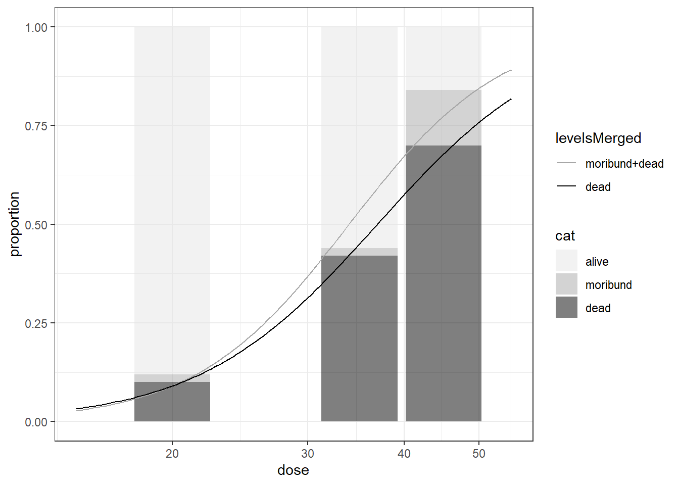

Code

bmdOrdinal(guthionS.LL, bmr = 0.1, backgType = "modelBased", def = "excess")

                   BMD     BMDL
moribund+dead 20.50104 17.11484
dead          20.59249 16.69573

Ordinal Regression in General

limited information and pertaintially unequal intervals, which requires a clear understanding of its subtleties and complexities, and careful attentions when implementing regression modelling.
Proportional Odds Model and Continuation Ratio Model, are standard regression models looking at ordered categories and transitions between them
Proportional Odds Model: Coefficient (slopes) remains constant across all categories.
Continuation Ratio Model: Model cumulative odds ratios.
Adjacent Categories Model: useful when neighboring categories influence each other.

[^1] (Pinheiro & Bates, “Mixed-Effects Models in S and S-PLUS”, Springer, 2000, pp. 163. )